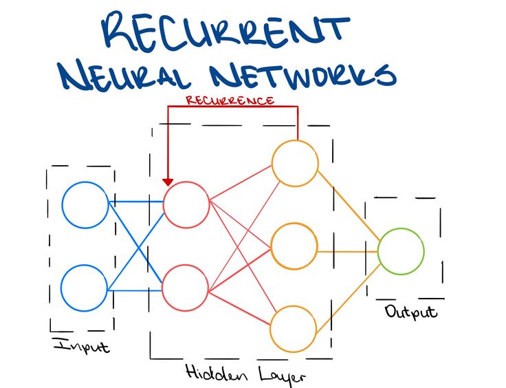
递归神经网络
简单的神经网络由三部分组成:输入,隐藏层,输出
深度神经网络(DNN)一般是增加隐藏层的数量。
递归神经网络(RNN)更加关注的是隐藏层中每个神经元在时间上的成长与进步。
Back Propogation Through Time
在普通的前馈神经网络 (feed-forward nn) 中,我们可以直接应用反向传播来计算梯度并更新权重。但是在 RNN 这种具有时间依赖的网络中,当前的输出不仅依赖于当前输入,还依赖于过去的隐藏状态。这就导致了参数的梯度计算需要沿时间维度进行传播,而 BPTT 正是解决这一问题的方法。 数学推导如下:
(1) 设定符号
- 输入序列:$ X = ${$x_1, x_2, …, x_T$}
- 输出序列:$ Y = ${$y_1, y_2, …, y_T$}
- 隐藏状态:$ h_t $ 表示时间步 $ t $ 的隐藏状态
- 参数:
- $ W_{xh} $:输入到隐藏层的权重
- $ W_{hh} $:隐藏层到隐藏层的权重
- $ W_{hy} $:隐藏层到输出的权重
- 损失函数:$ L(Y, \hat{Y}) $(如 MSE 或交叉熵)
(2) RNN 的前向传播 在 RNN 中,每个时间步的计算如下: $$ h_t = f(W_{hh} h_{t-1} + W_{xh} x_t) $$ $$ \hat{y} _ t = g(W_{hy} h_t) $$ 其中:
- $ f $ 是隐藏状态的激活函数(如 tanh 或 ReLU)
- $ g $ 是输出层的激活函数(如 softmax)
总损失为: $ L = \sum_{t=1}^{T} L_t(y_t, \hat{y}_t) $
(3) 反向传播 Through Time
计算损失对输出的梯度 $ \frac{\partial L}{\partial \hat{y} _ t} = \nabla_{\hat{y}_t} L_t $ 计算损失相对于输出的梯度,这部分和普通 BP 计算类似。
计算损失对隐藏状态的梯度 $ \frac{\partial L}{\partial h_t} = \frac{\partial L_t}{\partial h_t} + \frac{\partial L_{t+1}}{\partial h_t} + \frac{\partial L_{t+2}}{\partial h_t} + \dots $ 由于隐藏状态 $ h_t $ 会影响后续的所有时间步,因此梯度要沿时间方向反向累积。
计算参数的梯度
- 对隐藏状态的权重 $ W_{hh} $: $ \frac{\partial L}{\partial W_{hh}} = \sum_{t=1}^{T} \frac{\partial L}{\partial h_t} \cdot \frac{\partial h_t}{\partial W_{hh}} $
- 对输入权重 $ W_{xh} $: $ \frac{\partial L}{\partial W_{xh}} = \sum_{t=1}^{T} \frac{\partial L}{\partial h_t} \cdot \frac{\partial h_t}{\partial W_{xh}} $
- 对输出权重 $ W_{hy} $: $ \frac{\partial L}{\partial W _ {hy}} = \sum _ {t=1}^{T} \frac{\partial L}{\partial \hat{y} _ t} \cdot \frac{\partial \hat{y} _ t}{\partial W_{hy}} $
反向传播回传梯度
- 计算 梯度传播路径,从损失 $ L $ 反向通过时间步 $ T \to 1 $ 逐步更新参数。
- 使用 梯度下降(SGD, Adam) 来更新权重。
显而易见,BPTT存在两个致命问题:
- 第一个是梯度消失或爆炸:当权重矩阵的范数$||W_{hh}||$小于1时,随着时间步的增加,梯度指数级衰减,导致早期时间步的梯度几乎为 0,无法有效训练;
- 可能的解决方案:使用梯度裁剪(Gradient Clipping) 来限制梯度大小;使用长短时记忆网络(LSTM)或 门控循环单元(GRU) 代替 RNN。
- 第二个问题在于计算开销:BPTT 需要存储所有时间步的隐藏状态,因此当序列很长时,训练效率低。
- 可能的解决方案:Truncated BPTT,仅在固定窗口大小内进行梯度传播,而不回溯整个序列。
BPTT Variation
Truncted BPTT
- 策略:不展开整个时间序列,而是仅在 固定窗口大小 $ k $ 内进行反向传播(如$ k=10 $)。
- 优点:减少计算量,适用于长序列训练。
- 缺点:可能导致长程依赖信息丢失。
Online BPTT
- 计算一个时间步的梯度 立即更新参数(类似在线学习)。
- 适用于 流式数据处理(如语音识别)。
RNN Variation
LSTM 和 GRU 是RNN的两种主要变体,它们被设计用于解决传统RNN的梯度消失和梯度爆炸问题,从而更好地捕捉长程依赖(long-term dependencies)。LSTM和GRU可以通过门控机制(Gates) 控制信息流动,能够选择性保留或遗忘信息,有效缓解梯度消失问题,从而更好地学习长程依赖。
LSTM
(1) 结构
LSTM 主要引入了三个Gates和一个记忆单元(Cell State, $ C_t $):
- 遗忘门(Forget Gate):决定丢弃多少过去的信息。
- 输入门(Input Gate):决定更新多少新信息到记忆单元。
- 输出门(Output Gate):决定输出多少隐藏状态。
完整计算流程: $$ f_t = \sigma(W_f [h_{t-1}, x_t] + b_f) $$ $$ i_t = \sigma(W_i [h_{t-1}, x_t] + b_i) $$ $$ \tilde{C} _ t = \tanh(W_c [h_{t-1}, x_t] + b_c) $$ $$ C _ t = f _ t \odot C _ {t-1} + i _ t \odot \tilde{C} _ t $$ $$ o_t = \sigma(W_o [h_{t-1}, x_t] + b_o) $$ $$ h_t = o_t \odot \tanh(C_t) $$
(2) 详细解释
- 遗忘门 $ f_t $:控制是否遗忘过去的记忆。
- 输入门 $ i_t $:控制是否写入新的信息。
- 候选记忆 $ \tilde{C}_t $:当前时间步的新信息。
- 记忆单元 $ C_t $:更新后的长程记忆,信息可以直接在时间轴上流动,不易丢失。
- 输出门 $ o_t $:决定隐藏状态 $ h_t $ 的输出。
$ C_t $ 直接通过加法连接,使得梯度流动不会因多次乘法而消失。
GRU
GRU 是 LSTM 的简化版本,去掉了独立的记忆单元 $ C_t $,仅使用隐藏状态 $ h_t $ 作为存储信息的介质。
(1) 结构 GRU 主要有两个门:
- 重置门(Reset Gate):控制如何结合新的输入和过去的隐藏状态。
- 更新门(Update Gate):控制多少过去的信息保留,多少新信息加入。
完整计算流程: $$ r_t = \sigma(W_r [h_{t-1}, x_t] + b_r) $$ $$ z_t = \sigma(W_z [h_{t-1}, x_t] + b_z) $$ $$ \tilde{h} _ t = \tanh(W_h [r_t \odot h_{t-1}, x_t] + b_h) $$ $$ h_t = (1 - z_t) \odot h_{t-1} + z_t \odot \tilde{h} _ t $$
(2) 详细解释
- 重置门 $ r_t $:决定是否遗忘过去的隐藏状态。
- 更新门 $ z_t $:决定新旧信息的混合比例,类似 LSTM 的输入门和遗忘门的结合。
- 候选状态 $ \tilde{h}_t $:新的信息。
- 最终隐藏状态 $ h_t $:
- 当 $ z_t $ 逼近 1:当前状态 接近新信息。
- 当 $ z_t $ 逼近 0:当前状态 保留过去的隐藏状态。
GRU 用更新门合并了 LSTM 的输入门和遗忘门,因此计算更简单。
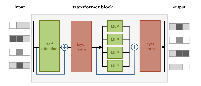
Transformers
虽然 LSTM 和 GRU 仍然被广泛使用,但现代NLP任务大多采用 Transformer(基于自注意力机制),因为:
- Transformer 并行计算 性能更强,而 LSTM/GRU 依赖序列处理,无法并行。
- Transformer 通过 Self-Attention 直接建模长程依赖,而LSTM/GRU仍然有一定信息衰减问题。
但在语音处理、时间序列预测等任务中,LSTM/GRU仍然具有较好的表现。
Self-Attention
The fundamental operation of any transformer architecture is the self-attention operation 1.
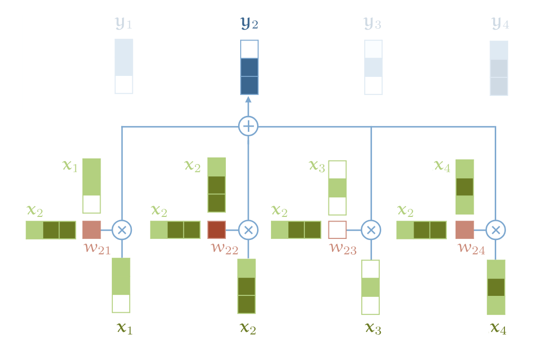
自注意力机制是一个从序列到序列的操作,它的输入是一组向量 $x_1, x_2, …, x_t$,对应的输出序列是 $y_1, y_2, …, y_t$。(每个向量都是k维)
每一个 $y_i$ 是怎么计算的?$y_i$是根据当前位置的$x_i$和其他所有位置的$x_j$的相关性计算出来的,具体公式如下 $$y_{\color{red}{i}} = \sum_{\color{blue}{j}} w_{\color{red}{i}\color{blue}{j}} x_{\color{blue}{j}}$$
对于$w_{\color{red}{i}\color{blue}{j}}$, 它是由$x_{\color{red}{i}}, x_{\color{blue}{j}}$的点积函数推导出来的。 $$w_{\color{red}{i}\color{blue}{j}} = \text{softmax}(w^{\prime}_{\color{red}{i}\color{blue}{j}})$$
其中 $$w^{\prime}_{\color{red}{i}\color{blue}{j}} = x^T_ix_j$$
原理可视化如下图所示,值得注意的是,这是整个体系结构中唯一在向量之间传播信息的操作。
为什么self-attention机制如此有效?我们拿电影推荐系统来举例子。假设你经营一家电影租赁公司,你有一些电影和一些用户,你想向你的用户推荐他们可能会喜欢的电影。一种方法是为电影手动创建特征,例如电影中有多少浪漫情节,有多少动作场面,然后为用户设计相应的特征:他们有多喜欢浪漫电影,有多喜欢动作片。如果这样做,两个特征向量之间的点积就会为电影属性与用户喜好的匹配程度打分。如果用户和电影的某个特征的符号相匹配–电影很浪漫,用户喜欢浪漫,或者电影不浪漫,用户讨厌浪漫–那么得到的点积就会得到该特征的正值。如果符号不匹配–电影浪漫而用户讨厌浪漫,则相应项为负值。
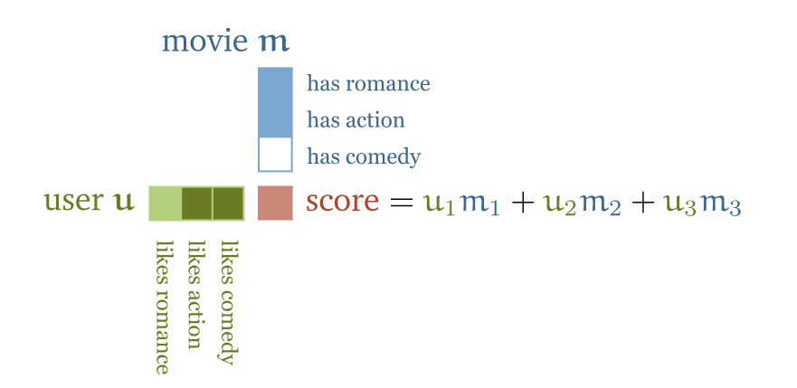
当然这样做并不现实,因为这涉及到大量的数据标注工作。一种解决办法是我们将电影特征和用户特征作为模型的参数,让用户选择一些喜欢的电影,然后通过优化算法调整用户特征和电影特征,使它们的点积能够匹配用户的已知喜好。即使我们没有告诉模型这些特征的具体含义,但在训练后,这些特征往往会自发地映射到有意义的电影内容信息。 例如,某个维度可能对应“浪漫”,另一个维度可能对应“动作”或“喜剧”,即使我们事先并未明确这些维度的含义。
这就是self-attention机制。它本质上是一种计算序列内部关系的方法。在处理文本时,我们首先为每个单词分配一个可学习的嵌入向量(embedding vector),例如句子 “the cat walks on the street” 会被映射为向量序列 $ v_{\text{the}}, v_{\text{cat}}, v_{\text{walks}}, v_{\text{on}}, v_{\text{the}}, v_{\text{street}} $。然后,这些向量进入self-attention layer,输出新的向量序列 $ y_{\text{the}}, y_{\text{cat}}, y_{\text{walks}}, y_{\text{on}}, y_{\text{the}}, y_{\text{street}} $。其中,每个 $ y_t $ 都是输入向量的加权和,而权重是根据归一化 (softmax) 的点积(dot product) 计算得到的。点积衡量了单词之间的相关性,如果两个单词在上下文中紧密相关,它们的点积就会较高,从而获得更高的注意力权重。例如,在句子中,“walks” 这个动词需要与“cat”建立联系,所以 $ v_{\text{walks}} $ 和 $ v_{\text{cat}} $ 的点积会较高,而“the” 这样的冠词由于对整体语义影响较小,通常不会与其他词有很大的点积值。
有趣的是,基础的self-attention并不关心输入的顺序,它只关注单词之间的相对关系。如果我们对输入序列进行重新排列,输出的向量序列也会以相同的方式被调整,而不会改变内容本身。这意味着自注意力本质上是一种集合操作(Set Operation),它不会依赖词的前后顺序,而是让模型自己学习哪些单词之间应该有更强的联系。此外,基础的自注意力层没有可训练参数,它的行为完全取决于输入向量,而这些向量来自于嵌入层,而嵌入层是可学习的。在完整的 Transformer 结构中,我们会通过位置编码(Positional Encoding) 让模型感知单词的顺序信息,但在纯自注意力层中,它是完全顺序不敏感的。
Query, Key, Value
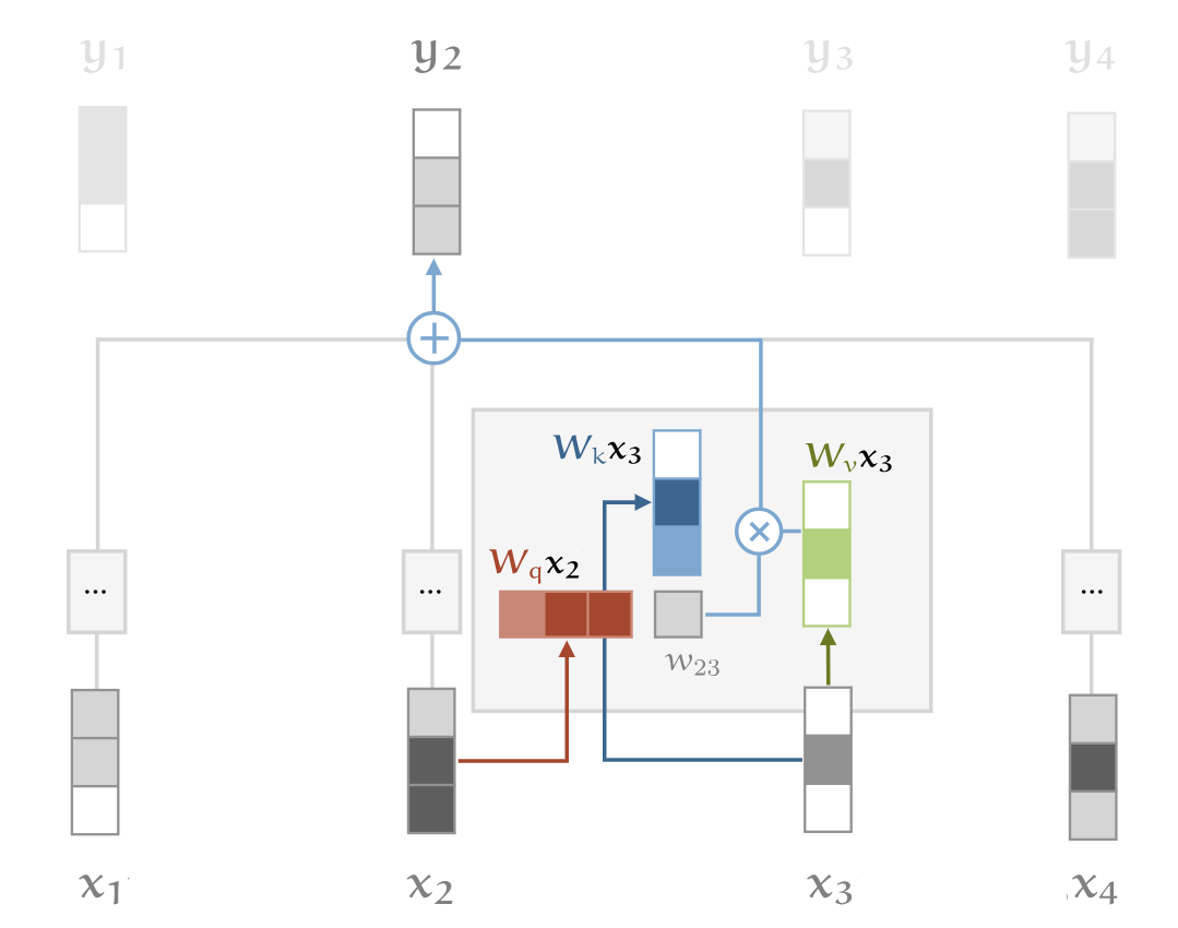
当代transformer中使用的self-attention还依赖三个额外的技巧 - Queries, Values, Keys。在 自注意力 计算中,每个输入向量 $ x_i $ 需要在三种不同的角色之间切换:
- 查询(Query,$ q_i $):每个词向量都需要与其他词向量进行比较,以确定它对自己的输出 $ y_i $ 的影响权重。
- 键(Key,$ k_i $):每个词向量也被其他单词用来计算权重,即它对其他单词输出 $ y_j $ 的影响。
- 值(Value,$ v_i $):在计算完权重后,每个单词的最终表示是所有词向量的加权和,其中加权方式由查询和键计算得到的注意力权重决定。
为了更方便计算,我们不会直接使用原始输入向量 $ x_i $,而是对其进行三次不同的 线性变换,得到: $$ q_i = W_q x_i, \quad k_i = W_k x_i, \quad v_i = W_v x_i $$ 其中 $ W_q, W_k, W_v $ 是可训练的 权重矩阵,用于学习适合任务的注意力表示。
接下来,计算两个词之间的相似性(相关性): $$ w’ = q_i^T k_j $$ 然后进行 softmax 归一化 以获得最终的注意力权重: $$ w_{ij} = \text{softmax}(w’) $$ 最后,每个单词的输出向量$ y_i $是所有值向量的加权和: $$ y_i = \sum_j w_{ij} v_j $$ 这个过程让模型能够动态调整单词之间的相互影响,从而更好地理解序列中的语义关系。
点积缩放
刚才我们使用 dot product 计算查询(Query)和键(Key)之间的相似性,并将其输入 Softmax 计算注意力权重。然而,当嵌入维度 $ k $ 较大时,点积的值会变得很大,导致 Softmax 的梯度变得极小,甚至造成梯度消失,影响模型训练。
为了解决这个问题,我们对点积进行缩放 (scaling dot product),即除以 $ \sqrt{k} $: $$ w’_{ij} = \frac{q_i^T k_j}{\sqrt{k}} $$ 从而防止输入值过大,使 softmax 函数输出的梯度保持稳定,提高训练效率。这样缩放的原因在于 高维向量的欧几里得长度随着维度 $ k $ 增大而增大,通过除以 $\sqrt{k}$,可以消除这种放大效应,使不同维度的计算结果保持在合理范围内,从而更稳定地学习注意力权重。
Multi-head Attention
在Self-Attention机制中,每个单词都可以与句子中的其他单词建立关系。然而,在标准的单头注意力(Single-Head Attention)机制下,一个单词只能用一个注意力分布来表示它与所有其他单词的关系。这就导致了一个问题:单个词可能在不同的上下文中承担不同的语义角色,但单头注意力无法区分这些角色。例如Mary gave roses to susan. 在 single-head attention 机制中,所有这些信息都会被简单地加权求和,而不会分别处理不同的语义关系。这意味着,“Mary” 和 “Susan” 都会影响 “gave” 的表示,但它们的影响方式是相同的,无法区分"施事者" 和 “受益者” 的不同语义。
多头注意力如何解决这个问题? 多头注意力(Multi-Head Attention) 通过使用多个独立的注意力头(attention heads) 来提供更高的表达能力。具体来说,每个注意力头(head)具有自己独立的查询、键和值变换矩阵:$W_q^r, W_k^r, W_v^r$,其中$r$表示不同的注意力头。对于输入$x_i$,每个注意力头都会产生一个输出向量$y_i^r$,把这些向量拼接起来,然后通过一个线性变换把维度降到k。
什么是Transformer?
Any architecture designed to process a connected set of units—such as the tokens in a sequence or the pixels in an image—where the only interaction between units is through self-attention.
下面是一个比较基础的架构
BERT
BERT - Bidirectional Embedding Representation Transformer
BERT与GPT架构的区别
Parsing
Decoding with LLMs
One naturally wonders if the problem of translation could conceivably be treated as a problem in cryptography. When I look at an article in Russian, I say: ’This is really written in English, but it has been coded in some strange symbols. I will now proceed to decode.
Terminology: continuation - 补全
我们如何生成the most probable continuation? $$ \arg\max_{w_1, …, w_n} p(w_1, …, w_n | \text{prefix}) $$ 如何求解?
- 遍历所有可能的续写,计算它们的概率,然后选择概率最大的那个。 但在自然语言处理中,可能的序列数量是指数级增长的,所以这种方法通常不可行。
- 另一种策略是逐步生成,即每一步选择当前最优的下一个单词(或 top-k 选项)。这种方法更实用,比如贪心解码(greedy decoding)
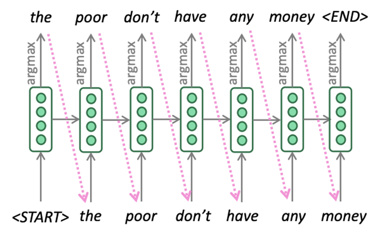
Greedy Decoding
下面是greedy decoding的具体流程
 这种解码方式的问题:
- 我们只做一次continuation,一旦发生错误无法回溯更改。
Beam Searching Decoding
根据greedy decoding的教训,我们选择保留几个continuation,并且每次都扩展most promising的那个。流程如下图所示
 Beam Searching如何实现?
- 用优先队列这样的数据结构来存储每个continuation
- 这个队列中保持最多k个解析
- 当要解码一个单词时,从队列中pop出一个解析,扩展完再push回队列
- 用priority queue这种结构来做,时间复杂度不会超过O(logk),甚至能达到O(1)
队列规模k的影响
- 当k=1,就是greedy decoding。所以当k较小时,我们会出现类似的问题
- 当k很大时,一方面是计算昂贵,一方面是有工作表明较大的k往往导致worse translation 2, 3。
- 而且当k很大时,往往生成的contination都很短,因为较短的continuation一般都是优选
- 因此,选择一个合适的k非常重要
解决方法:
Sampling
与其每次选择概率最大的,不如从输出的概率分布中采样。例如Top-k Sampling和Nucleus sampling
Holtzman et al. 对比了几种方法的效果,如图所示4
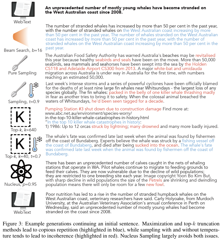
除此以外,还有Locally Typical Sampling
Top-k Sampling vs. Nucleus Sampling vs. Locally Typical Sampling
这些都是文本生成任务中用于解码(decoding)的策略,旨在平衡多样性和合理性,特别是在语言模型(如 GPT、LLM)中应用。
它们的核心目标是避免单一确定性输出(如 Greedy Search),让生成文本更加自然和富有变化。
核心思想:
- 选择那些使得模型生成的下一个单词在上下文中最符合“局部典型性”的单词。
- 不只是看单词概率本身,而是看它是否在上下文中“听起来”合理(局部熵最小)。
流程:
- 计算所有单词的概率 $ p(w \mid \text{context}) $。
- 计算这些单词的 信息熵(self-information): $$ s(w) = -\log p(w \mid \text{context}) $$
- 选择信息熵最接近平均信息熵(典型熵) 的一部分单词。
- 在这个子集中进行采样。
优点:
- 避免了 Top-k 和 Nucleus Sampling 的局限,使得输出更加符合上下文,而不是仅仅基于全局概率高低。
- 适用于对局部语境要求高的任务,比如对话生成、摘要等。
缺点:
- 计算复杂度略高,需要额外计算信息熵。
采样的目的就是平衡多样性和合理性。避免语言模型单一确定性的输出。
Neural Parsing
先复习下Encoder-Decoder架构,如下图所示,Encoder作用是将输入序列(如德语句子)编码成一个固定长度的上下文向量(context vector)。
- 输入词(如 “natürlich”, “hat”, “john”, “spaß”)首先被映射成词向量($ x_1, x_2, x_3, x_4 $)。
- 这些词向量依次输入到一个RNN 编码器(通常是 LSTM 或 GRU),产生隐藏状态 $ h_1, h_2, h_3, h_4 $。
- 这些隐藏状态捕捉了句子的信息,最终最后一个隐藏状态(这里是 $ h_4 $)被用作整个输入句子的上下文向量(context vector)。
Decoder接收编码器提供的上下文信息,然后逐步生成目标语言的句子(如英文)。
- 编码器最后的隐藏状态被传入解码器的 RNN 作为初始状态。
- 解码器使用 RNN(LSTM/GRU)逐步生成目标语言的单词:
- 初始状态 $ s_1 $ 依赖于编码器的最后一个隐藏状态。
- 每个时间步,解码器的 RNN 生成一个新的隐藏状态 $ s_t $。
- 通过一个 softmax 层,$ s_t $ 计算当前时间步的输出词 $ y_t $(如 “of”, “course”, “john”, “has”, “fun”)。
- 解码器的输出作为输入传递到下一步,直到生成完整句子。

Parsing is the task of turning a sequence of words
问题来了,句子解析的输入是一个序列,但输出不是,那我们如何用encoder-decoder模型来进行parsing?
我们可以linearize the syntax tree. 这样我们就有一个序列来表示输出了。例如:I saw a man with a telescope的句子解析就是
(S (NP (Pro You ) ) (VP (V saw ) (NP (Det a ) (N man ) (PP (P with ) (Det a ) (N telescope ) ) ) ) )
此外,还需要一些优化
- 添加EOS。使解码器知道何时停止生成,而不会一直无限制地预测单词。
- 反转输入字符串可以带来小幅的性能提升。
- 加深网络层数。例如对encoder和decoder都使用三层LSTM5。
- 添加注意力机制
- 使用word2vec作为输入(预训练的词嵌入)
- 自动生成训练数据,而不需要人工标注。Vinyals et al. (2015) 5 采用 Berkeley Parser(一个已有的句法解析器)来解析大量文本,并用这些解析结果作为训练数据。
可能发生的问题(比例很小,无需担心):比如我们如何确定opening and closing brackets match? 如何对应输入和输出?如何确保模型输出的是整个序列的最优parsing而不是仅仅预测每个time step上的best symbol?
Parsing with Transformers
Kitaev等人用transformers进行parsing。
- Use a transformer to encode the input
- This results in a “context aware summary vector” (embedding) for each input word.
- The embedding encodes word, POS tag, and position information.
- The embedding layers are combined to obtain span scores
- But they also try factored attention heads, which separate position and content information.
什么是span scores? 在NLP中,尤其是命名实体识别(NER)、句法解析(Parsing) 和 信息抽取(IE) 等任务中用于评估模型性能的指标。 Span scores 通常基于 Precision(精确率)、Recall(召回率) 和 F1-score(F1 分数) 来评估模型在 span-level 的表现:
Span scores在Transformer解析任务中的计算方法:计算span相关的向量差值,经过线性变换、归一化(LayerNorm)、非线性激活(ReLU)和再次变换,得到 span scores。最终,这些得分用于解码(decode the output),即找到最优的解析树。
Unsupervised Parsing
Unsupervised Parsing6主要是从未标记的文本中归纳出语法结构。
Unsupervised Parsing的SOTA的F-score只有60,对比supervised parsing来说很难,supervised parsing的F-score可以达到95以上
LLM前沿研究
Scaling Law
例如,给定固定的计算资源预算,训练Transformer语言模型的最佳模型大小和训练数据集大小是多少?
这类问题就可以用Scaling laws来回答。它提供了Compute Budget(C),size of model(N)以及number of training tokens(D)之间的一种关系。有一个粗略的共识是,它们可以使用power laws或类似的定律(以及它们的组合)来建模。
Power Law
Power Law描述的是变量x和它某些行为之间的关系,公式表示为$f(x) = \alpha x^\mathcal{-K}$
它有一个重要的性质:当$x$乘以一个因子时,$f(x)$也同样作为$κ$的函数乘以一个因子。即: $$ f(cx) = \alpha (cx)^\mathcal{-K} = c^\mathcal{-K}f(x) $$
Kaplan et al. (2020)
Kaplan等人的研究7总结
- 模型的性能很大程度上取决于scale(模型参数的数量,数据集大小,计算预算)而不是网络拓扑(层数,每层的宽度)。
- 数据集大小和模型大小的一起增长是很重要的。
- 性能可以用power law来建模。
还有一点,我们使用floating-point operations per second (FLOPs) 来衡量compute,而不是单纯依赖时间来衡量。
对他们的工作(Kaplan Scaling Law)的主要批判点在于,他们在训练中使用了相同的学习率。
Hoffmann et al. (2020)
以前的scaling law认为,增加计算预算(compute budget)时,优先增加模型大小(model size),其次才增加数据量(data size)。 比如计算预算 ×100 时,模型参数量 ×25,数据量 ×4。因为直觉上更大的模型能更有效地利用数据,所以数据规模的增长不需要太快。 但是,过度增加模型大小可能会导致过拟合或计算资源浪费。
Hoffmann等人2022年的研究提出了一个新的结论8:
计算预算增加时,模型大小和数据量应该同比例增长。 比如计算预算 ×100 时,模型大小 ×10,数据量 ×10。因为之前的策略导致很多大模型在小数据上训练,出现欠训练(undertrained models) 的问题。 Hoffmann 发现,更大模型并不一定能完全利用固定数量的数据,合理增加数据量可以显著提升模型性能。这个发现也影响了后续 LLM 训练策略,例如 GPT-4、Gemini、PaLM 等更关注 数据与模型规模的均衡增长。
如何推导Hoffmann等人提出的Chinchilla’s Scaling Law?
- L: LM average test loss (entropy loss)
- D: dataset size, number of tokens
- N: number of parameters
- C: compute budget, C=C(N, D) 已知一个固定的compute budget C*, 找到 $$ \arg\min_{N, D}L(N, D) = C^* $$ 用power law来建模: $$ L(N, D) = \frac{a}{N^\alpha} + \frac{b}{D^\beta} + c $$ $c$是理想的test loss
因此,Hoffmann等人训练出来了两个模型:
- Gopher: 280 billion parameters, 300 billion tokens, L(N, D) = 1.993
- Chinchilla: 70 billion parameters, 1.4 trillion tokens, L(N, D) = 1.936
Chinchilla 遵循这一策略(较小模型 + 更多数据),结果证明它在test loss和下游任务上表现更优。
增加效率
语言模型的训练中,主要做的计算就是矩阵乘法和求和归一化(Softmax)。用一个公式概括Transformer做的事情就是$\text{Softmax}(QK^T)V$
GPU是并行处理器,结构如下图所示
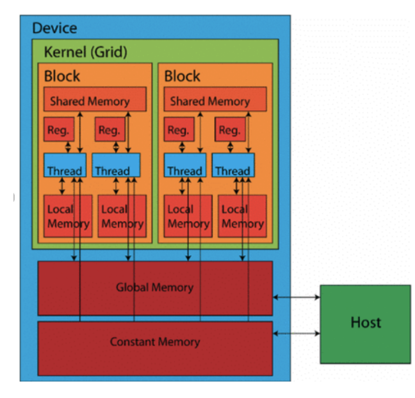
- 基础的计算单元是线程
- 线程被分组成Block,Block中的所有线程都有唯一的ID,但运行相同的代码
- 这使得GPU可以做极端的并行化
- Grid是一组Block。每个Block可以运行不同的代码段
- GPU有很大的global memory,很大,但是很慢
- 每个Block都有一个共享内存-Block中的所有线程之间共享这个内存,它效率很高,但很小
- 写代码时要尽可能少用全局内存,多用Block的共享内存
Double Descent
Double Descent是深度学习训练过程中出现的一种现象,它描述了模型的test error随着model size或dataset size变化的非单调趋势。 Double Descent 现象表明,在“过拟合区域”之后,继续增加模型规模,test error反而会再次下降,进入“第二次泛化区域”。
因此,传统统计学习理论预测过拟合会导致泛化能力下降,但Double Descent说明在超大模型下,泛化能力反而会回升。
LLMs as Formal Machines
一个自回归语言模型定义$p(y)$ $$ p(y) = p(\text{EOS}\mid y)\prod_{t=1}^n p(y_t \mid y_{<t}) $$
模型不是直接在文本上建模,而是先把上下文变成一个向量(representation),再在这个向量上建立条件概率分布,预测下一个词。 $$ p(y_t\mid y_1, …, y_{t-1}) = \text{Softmax}(Eh(y_1, …, y{t-1}))_{y_t} $$
$h(y_1, …, y{t-1})$是历史上下文经过模型(比如 Transformer)编码后的隐状态(hidden state)。是词表 embedding 矩阵,通常大小是$V\times d$,$V$是词表大小,$d$是embedding维度。这里是output projection,也就是把隐状态投影回词表空间,生成每个词的得分。最后Softmax函数把所有词的得分归一化成概率分布(每个词一个概率)。
LLM如何通过formal language theory角度来理解?
- FSM → PDA → TM → LLM
- LLM本质上在定义一种语言,也就是定义“哪些字符串是合法的”。
- Formal Language Theory把LLMs看成一类接受语言的机器,研究它们能接受(或生成)多复杂的语言,从而理解它们的计算能力和局限。
机器 | 本质上在做什么? | 能接受什么样的语言? FSM(有限状态机) | 有有限个状态,读入符号,跳转状态,最后看是不是到达接受状态。 | 正则语言(比如模式识别:找有没有特定的词) PDA(下推自动机) | 有状态+一个栈,可以压栈/出栈,增加了“记忆”能力。 | 上下文无关语言(比如括号匹配:{(())()}{ (())() }{(())()}) TM(图灵机) | 有无限长的带子,可以读写,前后移动,状态转移,可以做任意复杂的操作。 | 递归可枚举语言(基本上 = 可计算的问题)
什么是可计算的语言?
- 有某种机械的方法(算法/程序)可以判定一个字符串是否属于这个语言。
Safety & Security with LLMs
- LLMs(大型语言模型)带来的安全和隐私风险
- 神经表征信息提取:攻击者可以尝试从模型隐向量中恢复敏感信息。
- 成员关系攻击(membership attacks):判断某个样本是否出现在训练集中。
- 模型蒸馏/盗窃(model theft):通过访问接口,训练出性能接近的大模型(例如Vicuna从ChatGPT)。
- 越界输出:诱导模型输出非法或敏感内容。
- 滥用模型:比如利用模型生成虚假信息、代写论文等。
- 水印(Watermarking)技术
- 原理:通过在模型生成过程中对词表分组(绿牌词、红牌词),让模型偏好生成绿牌词,从而在输出文本中嵌入人类不可察觉但可机器检测的“隐形签名”。
- 检测方法:检验文本中出现红牌词的数量,进行统计检验(若文本自然生成,红牌词出现概率应为50%;若有水印,红牌词出现次数极少)。
- 局限性:
- 低熵情形下(可选词很少)难以有效植入水印。
- 经第三方**改写模型(paraphrasing)**处理后,水印可能被破坏。
- 越狱攻击(Jailbreaking)和对抗性提示(Adversarial Suffix)
- Zou et al. (2023)提出的方法:
- 通过给提示词后面添加一个特定后缀,可以让模型忽视原有的安全限制,输出被禁止的信息。
- 他们用梯度指导的离散优化搜索这种对抗性后缀(对token的one-hot向量求梯度,选择影响最大的新词替换)。
- 通用后缀(Universal Prompt):
- 研究发现,找到的一些后缀不仅能攻击开源模型(如Vicuna),还可以迁移攻击闭源模型(如GPT系列)。
- 局限:不需要完全的模型访问(黑盒攻击可能有效)。
- 公平性问题:保护敏感属性(比如性别、种族)
- 故事背景:Amazon曾因招聘系统偏见问题,希望模型在决策时不使用敏感属性。
- SVD信息擦除方法(Shao et al., 2023):
- 建立输入(X)与敏感属性(Z)的协方差矩阵。
- 对其做奇异值分解(SVD),然后将X投影到与Z正交的子空间,从而去除敏感属性的信息。
- 挑战:
- 在样本与敏感属性未一一对应(unaligned)时,如何做擦除?
- 可以通过推测潜在对应关系(latent alignment)部分实现。
- 总结
- LLMs存在多种安全隐患:信息泄露、不当使用、输出违法内容、不公平决策等。
- 水印、对抗攻击研究、信息擦除(保护隐私与公平)是当前重要的安全与伦理研究方向。
什么叫奇异值分解?将X投影到与Z正交的子空间为什么就可以去除铭感属性的信息?
奇异值分解(Singular Value Decomposition,简称 SVD)是线性代数里一个非常重要的矩阵分解方法。
它的基本形式是:
$$ M = U \Sigma V^\top $$
其中:
- $ M $ 是一个 $ m \times n $ 的矩阵(可以是非方阵)。
- $ U $ 是一个 $ m \times m $ 的正交矩阵(列向量是正交单位向量)。
- $ V $ 是一个 $ n \times n $ 的正交矩阵(列向量也是正交单位向量)。
- $ \Sigma $ 是一个 $ m \times n $ 的对角矩阵(对角线上的元素是奇异值,非负,且通常按降序排列)。
简单理解就是:
SVD把任意矩阵拆成了旋转 + 拉伸 + 再旋转三步过程的组合。
- $ X $:是用户的输入表示,比如文本、图像特征。
- $ Z $:是不希望模型依赖的敏感属性,比如性别、种族、年龄等等。
目标是:
希望模型在保留对 $Y$(正常任务)的预测能力的同时,尽量删除X中关于Z的信息。
为什么可以用SVD来去除敏感属性?我们可以这样操作:
计算协方差矩阵:
先计算$ X $和$ Z $之间的交叉协方差矩阵:$$ \Omega = E[X Z^\top] $$
这个矩阵描述了$ X $中每一维与$ Z $中每一维之间的线性关系。
对 $ \Omega $ 做SVD:
$$ \Omega = U \Sigma V^\top $$
其中:
- $ U $ 的列向量告诉我们:在$ X $空间中,哪些方向(组合)与$ Z $的变化最相关。
- 奇异值$ \Sigma $的大小表示这种相关性的强弱。
去除高相关方向:
- 将$ X $投影到与最相关方向正交的子空间。
- 就是:去掉$ U $中对应最大奇异值方向的分量,只保留剩下的。
- 具体地,新的$ X $(记作 $ X_{\text{erased}} $)是:
$$ X_{\text{erased}} = UU^\top X $$
其中$ U $是那些最小奇异值对应的正交基向量(跟敏感信息最不相关的方向)。 4. 为什么这种投影能去掉敏感属性的信息?
- $ \Omega $告诉我们哪里有“泄漏”,也就是$ X $哪些方向最容易揭示$ Z $。
- 投影到正交空间,本质上是抹掉了与敏感属性相关的变化方向。
- 直觉上理解:如果性别主要影响了特征的第一个方向,那我们就从表示里去掉这一方向的信息,剩下的内容就跟性别的相关性大大降低了。所以,去除这些方向以后,模型就难以再通过X推测出Z了,从而提升公平性。
LLM微调
GPT发展历史:
- GPT: 117M parameters, decoder-only model with 12 layers, trained on 4.6GB data
- GPT-2: 1.5B parameters, decoder-only model with 48 layers, trained on 40GB data
- GPT-3: 175B parameters, unkown model structure, trained on 600GB data
介绍下In-context learning, 是指LLM在不进行参数更新的情况下,仅通过输入示例来完成新任务。就是让模型“看例子学套路”而不是“调参数学规则”。但是这会让模型对提示词高度敏感,而且适用范围也受限
指令微调
- Collect examples of instruction-output pairs across several tasks and fine-tune a model, then evaluate on unseen tasks.
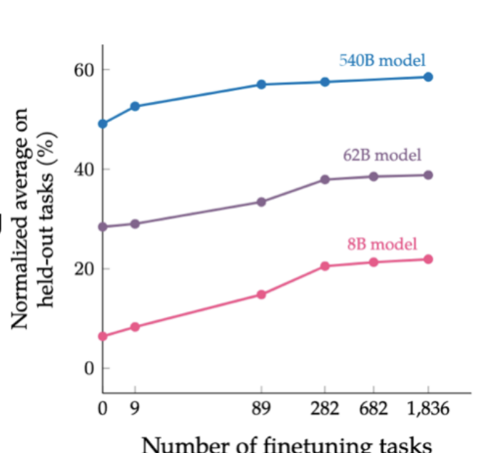 如图所示,可以说明:
- Model generation performance is positively correlated with observed tasks and model size.
- Number of examples does not have a big influence.
RLHF
Logic behind learning from human feedback
- Say we had human “rewards” – a score that tells how much a human prefers a completion. Say there is such function called $r(x, y)$ that maps prompt and completion to a reward
- We would want to find an LLM with parameters $\theta$ such that
$$ \theta = \arg \max_{\theta} \mathbb{E} _ {p _ {\theta}(x,y)}[r(x,y)] $$
- This is the model that maximises the expected reward according to humans.
问题来了,怎么更新参数?(怎么计算梯度?),因为reward函数是外部评估器,没办法直接对其求梯度。
首先定义$z = (x, y)$是一个完整的生成序列,那么要求: $$ \nabla_\theta \mathbb{E} _ {p_\theta(z)}[r(z)] = \nabla_\theta \sum_z p _ \theta(z) r(z) $$ 梯度更新$\theta$,$r(z)$与其无关,所以放进去: $$ = \sum_z r(z) \nabla_\theta p _ \theta(z) $$ 然后用log-derivative trick变换: $$ \nabla_\theta p_\theta(z) = p_\theta(z)\nabla_\theta \log p_\theta(z) $$ 所以替换过后就变成了 $$ \sum_z r(z) p_\theta(z)\nabla_\theta \log p_\theta(z) $$ 然后变成期望形式 $$ \mathbb{E} _ {p_\theta(z)}[r(z)\nabla_\theta\log p_\theta(z)] $$
用模型生成一些$(x_i, y_i)$,然后用打分函数得到$r(x_i, y_i)$,再去近似估计上面的期望 $$ \nabla_\theta \mathbb{E}[r(x,y)] \approx \frac{1}{n} \sum_{i=1}^n r(x_i, y_i) \nabla_\theta \log p_\theta(x_i, y_i) $$ 再用这个梯度来更新参数 $$ \theta_t \leftarrow \theta_{t-1} + \frac{\alpha}{n} \sum_{i=1}^n r(x_i, y_i) \nabla_\theta \log p_{\theta_{t-1}}(x_i, y_i) $$ $\alpha$是学习率,梯度更新本质上是用reward加权的log-likelihood梯度来更新。这样做之后,虽然我们不能对reward直接求导,但是可以让reward控制梯度的大小。
RLHF的问题是什么?是人类,人类标注不仅高成本,而且标注结果噪声不小。Bradley-Terry Model可以用来减少这个噪声
Bradley-Terry 模型是一种用于建模“成对比较”胜负概率的概率模型。当你有一堆对象(比如选手、商品、翻译结果),你观察到一堆"谁胜过谁"的比较对,这个模型可以帮你计算每个对象的强度分数。
我们希望通过人类偏好(human preferences)来训练一个奖励函数 $ r $,然后用这个奖励函数优化语言模型的行为。
设定:偏好数据集
Let $ (x_i, y_{1,i}, y_{2,i}) $ be the set of preferences
意思是:
- 每条数据包含:
- 一个输入 prompt $ x_i $
- 两个回复 $ y_{1,i} $ 和 $ y_{2,i} $
- 人类偏好告诉我们:“在这个输入下,更喜欢 $ y_{1,i} $ 胜于 $ y_{2,i} $"。
这构成了一个成对比较**,就像 Bradley-Terry 模型那样。
第一步:训练奖励函数 $ r $
Let $ R $ be a set of reward functions…
$$ r^* = \arg\max_{r \in R} \sum_i \log \sigma(r(x, y_{1,i}) - r(x, y_{2,i})) $$
这是在用人类偏好来训练 reward model,意思是:
- 用 sigmoid 函数 $ \sigma(\cdot) $ 估计偏好概率。
- 如果 $ r(x, y_1) $ 比 $ r(x, y_2) $ 高,就表示模型认为 y₁ 更好,和人类偏好一致。
- 目标是最大化所有数据上这个 log-likelihood 的和(类似 Bradley-Terry)。
最终得到一个最优奖励函数 $ r^* $,它可以打分“一个回复有多好”。
第二步:优化语言模型
Let $ P $ be the space of LLMs, then optimize:
$$ \max_{p \in P} \frac{1}{n} \sum_i \mathbb{E}{p}[r^*(x_i, y)] - \frac{\beta}{n} \sum_i D{\mathrm{KL}}(p(\cdot\mid x_i) | p_0(\cdot\mid x_i)) $$
这是一个训练目标:
用奖励函数 $ r^* $ 指导 LLM $ p $ 的更新,但同时限制它不能偏离原始模型 $ p_0 $ 太远。
解释:
- 第一项:希望新的模型 $ p $ 在每个输入 $ x_i $ 下,输出的 $ y $ 具有高 reward。
- 第二项:用 KL 散度惩罚项,确保新模型和原始模型 $ p_0 $ 不差太远。
- $ \beta $ 是一个超参数,控制两者权衡。
这就形成了一个reward-regularized objective,类似于 RLHF 中的 PPO 或 DPO 框架。
- 训练一个新的 LLM(叫 $ p $),它能更符合人类偏好(因为用了奖励函数 $ r^* $)。
- 但又不会和原来的 LLM $ p_0 $ 差太多,保证安全性、稳定性和保持原始能力。
但是我们真的需要reward吗?reward本质上等价于新旧模型概率差,直接用这个差值就能表达偏好。这就是DPO的核心思想
DPO将RLHF转换为基于偏好数据的微调问题
Summarising Text
Types of summarisation models:
- Multi-document versus single document
- Extractive versus abstractive
- Generic (unconditioned) versus query-focused (conditioned) or controllable
- Supervised versus unsupervised
- Multi-modal versus single modality
Multi-document summarisation vs Single-document summarisation
- Single document summarisation use a single source, for example, a news article
- Multi document summarisation uses multiple sources or documents for the summary (all sources are related to a theme or topic)
Query-focused summarisation vs Controllable summarisation
- Query-focused: summarise a document based on a specific query
- Controllable: Control parameters such as length, aspect, sentiment
Extractive summarisation vs Abstractive summarisation
- Extractive: use a subset of the sentences from the document as the candidate summary
- Abstractive: synthesise a summary which is not tied to the exact wording in the article
Extractive总结很简单:对于一个有n句话的文档$d=(s_1, s_2, …, s_n)$, 然后做分类,如果这个句子应该放在summarisation中,就是$y_i=1$,否则$y_i=0$。非常简单,但是是许多summarizer的基础模型。
对于二分标签总结,有两个问题
- 从哪里获得训练模型的标签?
- 训练目标是什么?朝什么方向优化?
对于标签,给定一篇文章(含多句子)和它的“参考摘要”。然后计算每句话和参考摘要之间的 ROUGE 分数(ROUGE 测的是和摘要重合的词/短语数量)。选出 得分最高的几个句子,作为模型的正样本(打上 1 标签),其他句子为0。
对于训练目标,现在每个句子都有一个标签(是否该被选进摘要),用 logistic 回归或者其他分类器,目标是最大化这堆标注的 log-likelihood。这就是标准的 binary cross-entropy: $$ \mathcal{L} = -\sum_i \left[ y_i \log p_i + (1 - y_i)\log(1 - p_i) \right] $$
Abstractive总结:这个问题应该被视为文本生成问题,而不是之前的选择问题。使用的是pointer-generator network。
- Base model是一个seq2seq架构(输入文章由encoder编码,输出摘要由decoder逐词生成)。
- 这个base model的问题是标准的seq2seq模型很难生成词表外的词,而且容易错过原文中的关键词
- 解决办法就是pointer-generator network,引入指针机制,这样每一步生成单词$w$的概率就变成了一个混合模型 $$ P(w) = p_{\text{gen}} P_{\text{vocab}}(w) + (1 - p_{\text{gen}}) \sum_{i: w_i = w} a^t_i $$
- 这个公式表示模型可以选择 “从词表中生成” 或 “从原文中复制”,通过$p_{\text{gen}}$来动态切换。
- 还有一个问题是这个模型通常生成重复内容,因此引入coverage vector $c^t = \sum^{t-1}_{t’=0}a^{t’}$
- 这个向量记录了过去decoder在source上的attention积累量,新一轮decoder中把这个vector输入进来可以防止过度关注同一个片段,从而减少重复。
ROUGE分数是什么?如何计算?
- ROUGE是Recall-Oriented Understudy for Gisting Evaluation,值越高越好。 $$ \text{ROUGE-N} = \frac{\sum_{S\in ref}\sum_{\text{gram} _ n\in S}\text{countmatch}(\text{gram} _ n)}{\sum_{S\in ref}\sum_{\text{gram}_n\in S}\text{count}(\text{gram}_n)} $$
- 为什么计算的是召回率而不是精确率?Recall is more important to decide whether the information in the candidate summary captures the information in the reference summary.
还有一种分数不依赖n-grams,用BERT来softly score similarity. 它计算的是语义相似度
- 使用BERT提取每个词的向量表示,再用余弦相似度比较候选摘要和参考摘要之间的每个词是否“语义接近”。
- 给定$C$是candidate sentence,$R$是reference sentence
- 用BERT把C和R中的每个词编码成向量。$C=[c_1, …, c_n], R=[r_1, …, r_m]$
- 每个词对之间都计算余弦相似度,得到一个 n×m 的相似度矩阵
- 每个词从对方句子中找最相似的词作为匹配,得到precision(每个生成词去参考里找最相似的词)和recall(每个参考词去生成中找最相似的词)两个方向的得分。最终的F1 score就是 $$ \text{BERT Score} = \frac{2 \times \text{Precision} \times \text{Recall}}{\text{Precision} + \text{Recall}} $$
PEFT
先夹带私货,欢迎关注我在LoRA as a Service (LaaS)方面的工作
假设有一个神经网络函数$ f: X \to Y $,可以表示为多个子函数的组合:
$$ f_{\theta_1} \circ \dots \circ f_{\theta_n} $$ 每个子函数$ f_{\theta_i} $有自己的参数$\theta_i$。我们希望通过一个只含有少量参数的模块$ \phi $来对这个网络进行微调(即 PEFT 的目标),而不是更新整个模型的参数$ \theta $。
PEFT分为三类
Parameter composition: $$ g_i(x) = f_{\theta_i \oplus \phi}(x) $$
- 用一个组合操作$ \oplus $将原始参数$ \theta_i $与微调模块参数$ \phi $融合。
- 举例:LoRA就是这种方式,它在原始权重上添加了一个低秩矩阵。
Input composition: $$ g_i(x) = f_{\theta_i}([x, \phi]) $$
- 把 $ \phi $ 拼接在输入$ x $上作为新的输入。
- 举例:Prefix Tuning就是这种方式,它把微调参数作为“前缀”输入到 Transformer 中。
Function composition: $$ g_i(x) = f_{\theta_i} \circ f_{\phi}(x) $$
- 把$ f_\phi $作为前置函数处理输入,再送入原始函数$ f_{\theta_i} $。
- 举例:Adapter 模块可以看作在主模型中插入了一个前置的小网络。
首先介绍三种常见的parameter composition实现方式
- Sparse network
- 让$\phi$具有稀疏结构,即只有一小部分参数是非零的。目标是减少计算和内存开销,同时保留表达能力。
- Structured composition
- 在原始参数$\theta_i$上施加结构化限制,例如只更新某些预定义结构中的参数(比如只调 Transformer 中的 FFN 或某层的 attention)。
- Low rank composition
- 把参数表示成低秩矩阵,比如将全连接层的权重调整部分限制为两个小矩阵相乘(低秩近似)。
| Parameter Efficiency | Training Efficiency | Inference Efficiency | Performance | |
|---|---|---|---|---|
| Parameter Composition | methods require <3% of params | pruning requires re-training iterations | does not increase model size | LoRA achieves strong performance |
| Input Composition | only add a small number of params | extend the context’s window | extend the context’s window | require large models to perform well |
| Function Composition | adapters depend on hidden size | does not require gradients of frozen params | new functions increase # of operations | mactch or outperform standard fine-tuning |
Evaluating Generation & Machine Translation
Evaluation Translation & Generation
- 为什么评估重要但困难
- 测试是工程中的核心部分。比如给你一个机器翻译系统,怎么判断它“对”呢?评估就是回答这个问题。
- 评估不仅要比较不同系统,还要监控系统迭代(新方法有没有改善)和判断系统是否适用于特定应用场景(比如翻译菜单 vs 翻译和平协议)。
- 人工评估
- 关键两个维度:
- Adequacy(充分性):翻译有没有完整传达原文意思?
- Fluency(流畅性):语言是否自然、符合语法?
- 人评的方式:给分(比如1-5分),但评审间经常存在分歧。
- 介绍了直接评估(Direct Assessment)的方法,比如用滑动条细致打分,提高一致性。
- 基于字符串重叠的自动评估
- 自动评估是为了快速检测系统变化,比如Google Translate更新时不能每次都靠人评。
- 最简单的方法是匹配单词,计算Precision/Recall/F1,但这样的问题是忽略了词序。
- 更先进的方法是BLEU(Bilingual Evaluation Understudy)分数:
- 统计n-gram(n个连续词)的匹配情况。
- 引入惩罚机制(比如翻译太短会扣分)。
- 缺点:对词形变化敏感,对内容的重要性不区分,难以跨数据集解释,且对人类翻译的得分也可能偏低。
- 使用Embedding的评估
- 传统指标很表面,无法处理同义表达、重要单词位置变化的问题。
- BERTScore:
- 用BERT等预训练模型的上下文嵌入来表示句子。
- 计算每个token之间的余弦相似度,进行贪婪匹配。
- 可以选择加入IDF(逆文档频率)加权,强调稀有重要词。
- 用训练出来的模型评估
- 通过收集16年WMT比赛的人类评估数据,训练模型来自动打分。
- 代表性方法是COMET:
- 用跨语言预训练模型编码源句、参考翻译和系统输出。
- 输入特征包括向量间的乘积和差值。
- 用回归模型(如MSE)来预测翻译质量分数。
- 比BLEU和BERTScore和人类判断的相关性更高。
- 总结
- 好的NLG/MT评估非常重要也非常难。
- 需要同时关注充分性(adequacy)和流畅性(fluency)。
- BLEU等传统指标有用,但局限明显。
- 训练出的新一代指标(如COMET)表现更好,但也要小心夸大其效果。
- 评估时应该使用多种指标、大且多样化的测试集和合理的人工评估者。
Machine Translation & Multilingual data
- 低资源机器翻译(Low-Resource MT)
- 什么是低资源?
指数据稀缺的语言,无法像英语、法语那样有大量双语或单语数据支撑NLP模型训练。 - 语言分类(根据资源多少):
- Class 0:完全被忽视的语言(如Dahalo)
- Class 1:有少量未标注数据(如Bhojpuri)
- Class 2:有极少量标注数据(如Zulu)
- Class 3-5:资源逐步丰富,如英文、德文等是Class 5“赢家”。
- 现实问题:
- 大量语言在数字世界中几乎没有存在感。
- 资源稀缺问题反映了社会性系统不公。
- 如何提升低资源语言MT
回译(Back Translation):
- 先训练一个反向翻译器(如英语→祖鲁语),再生成伪数据反向训练祖鲁语→英语。
- 迭代回译(Iterated Back Translation)可以进一步增强效果。
迁移学习(Transfer Learning):
- 使用资源丰富语言的平行语料来初始化低资源语言的系统。
- 父母语言不需要同源,比如用英语帮辅导斯瓦希里语。
mBART模型(Multilingual BART):
- 预训练:在25种语言的大规模单语数据上做降噪自编码训练。
- 微调:在小规模双语数据上进行具体翻译任务的微调。
- 效果:在低/中资源语言对上显著提升BLEU分数,但对高资源语言提升有限,甚至可能轻微下降。
mBART50:
- 扩展到50种语言。
- 支持多对多(many-to-many)翻译,不仅限于英↔X。
- 多语言翻译模型(Multilingual Models)
思路:
- 用一个模型支持多个语言对(比如103种语言互译),而不是为每一对单独训练。
好处:低资源语言受益于高资源语言(Transfer)。
问题:不同任务之间互相干扰(Interference),尤其是高资源语言性能可能受损。
解决方法:
- 平衡采样:通过调整训练样本分布(如温度采样),降低高资源语言对低资源语言的压制。
- 注入Adapter模块:在Transformer中插入小型adapter层,让不同语言任务可以独立调整,减少干扰。
- 低资源MT的评估问题
- 自动评估(如BLEU)对低资源语言来说更不可靠:
- 原因一:这些指标本身是为高资源系统设计的。
- 原因二:系统质量较差时,指标波动性大。
- 原因三:缺乏好的测试集和人类标注数据训练指标。
- 最佳实践:
- 尽量进行人类评估。
- 鼓励研究者直接联系语言社区,进行参与式研究。
- 总结
- 低资源MT已经取得明显进步,但世界上大多数语言依然未被很好支持。
- 研究重心逐步从传统encoder-decoder转向以LLM为基础的方案。
- 未来挑战依然很多,尤其是在知识注入、控制生成、多语言泛化等方面。
Translation & LLMs
Ethics
Ethics in NLP
- NLP的社会影响 Benefits
- Efficiency for individuals and institutions trying to understand and summarize information in many languages.
- Personalization for users, e.g. through digital assistants, tutoring agents, and other services.
- Human understanding of the language faculty and its social use—e.g. through use in computational psycholinguistics and computational sociolinguistics.
- Types of Risks
- Discrimination, Exclusion and Toxicity
- Information Hazards
- Misinformation Harms
- Malicious Uses
- 构建NLP系统时需要考虑的事情
- Advanced grammar analysis can improve search and educational NLP but also reinforce prescriptive linguistic norms and discrimination.
- Stylometric analysis can help discover provenance of historical documents but also unmask anonymous political dissenters.
- Text classification and IR can help identify information of interest but also aid censors.
- Machine translation can be used to break language barriers but also monitor marginalized populations.
Bias in word embeddings
- Bias in representations
词表示(Word Representations)中的偏见 人类有社会偏见,这些偏见也能通过隐性联想测试(IAT)测出来。类比地,**词向量(如GloVe、word2vec)**中也能检测到类似的偏见。比如:
- 男性名字更容易和“事业(career)”类词联系在一起。
- 女性名字更容易和“家庭(family)”类词联系在一起。
- 这种检测方法叫做 WEAT(Word Embedding Association Test)。
- Bias in NLP systems
偏见不仅存在于向量中,还影响了实际NLP应用。例如,在情感分析系统中(200多个模型参与测试):
- 黑人名字更容易被识别为“愤怒、恐惧、悲伤”。
- 白人名字更容易被识别为“快乐”。
性别上:
- 女性名字更容易和“愤怒、快乐”关联。
- 男性名字更容易和“恐惧”关联。
- 即使只改变人名,情感分类的输出也发生了显著变化,说明系统有人口统计偏见(demographic bias)。
- What can you do?
硬去偏(Hard Debiasing)
找到性别子空间(gender subspace),通过种子词对(如 he-she, man-woman)确定。把所有中性词(如doctor、teacher)沿这个子空间方向上的分量清除掉。
问题:这种方法只是简单地清除了某个方向的信息,但实际上偏见可能分散在很多维度上。研究发现,即使做了去偏处理,模型仍然能学到隐含的性别、种族等信息(Gonen and Goldberg, 2019)。
调整训练数据(Dataset Debiasing)
- 例如,在毒性检测任务中,如果某些词(如"gay”)在有毒评论中出现频率很高,那么可以通过增加无毒例子来平衡。这种方法对监督学习任务有效,但对文本生成(如LLMs)来说挑战更大。
价值对齐(Values Alignment)
- 使用针对社会价值观制作的数据集(比如PALMS项目),训练模型符合特定的道德立场(比如尊重多样性,反对性别刻板印象)。
解码时控制(DEXPERTS)
- 训练小模型作为“专家”和“反专家”,在大模型推理时组合控制输出。不需要重新训练大模型,非常高效。
In context learning
- 什么是 In-Context Learning(ICL)?
- 定义:通过在输入中提供任务示例((x, y)对),让模型学习任务规则;
- 不更新参数,纯靠 prompt;
- 举例:
text: Worst film ever target: negative - Few-shot / Zero-shot Learning 是 ICL 的应用形式。
- ICL 的局限性
- 对 prompt 很敏感:格式不佳、顺序不佳都能显著降低性能;
- 模板不易泛化:一个任务有效的模板可能在新任务中无效;
- 在复杂推理任务上效果差:
- 算术推理(AR)
- 常识推理(CR)
- 符号推理(SR)
- Chain-of-Thought Prompting(CoT)
- 定义:让模型通过“自然语言的逐步推理过程”来得到答案。
- 类似逻辑编程中的“反向链推理(backward chaining)”。
- 目的:
- 将复杂问题拆解成多个简单子步骤;
- 提供推理解释,增强透明度;
- 无需训练,只需写 prompt!
- CoT 的例子
普通 zero-shot(失败):
Q: 16个球,一半是高尔夫球,一半的高尔夫球是蓝色的。问多少个蓝色高尔夫球?
A: 8  ❌
CoT zero-shot:
A: Let's think step by step.
→ 一共16球 → 一半是高尔夫 = 8 → 一半的高尔夫球是蓝色 = 4  ✅
CoT 中的关键词是:
“Let’s think step by step.”
- CoT 的实验结果(Few-shot & Zero-shot)
| 模型规模 | CoT 效果 |
|---|---|
| <10B | 无明显提升 |
| >100B | 效果显著提升 |
- Few-shot CoT > Zero-shot CoT;
- 在 GSM8K、AQuA、SVAMP 等数据集上显著提高算术问题解决能力。
- Symbolic Reasoning 测试
测试模型处理“规则推理任务”的能力,如:
- 字符拼接(Last Letter Concatenation);
- 抛硬币推理(Coin Flip);
- 分析:CoT 在 OOD(更长步骤)测试上更稳健。
总结一句话:
ICL 是用“上下文中的例子”教模型做任务;而 CoT 则是教模型“按步骤思考”。尤其对于大模型,CoT 能显著提升复杂推理任务的表现。
Question Answering
- 什么是问答系统?
- 构建能够用自然语言自动回答人类提问的系统。
- 任务形式:给定一个问题(Q),输出答案(A)。
- 问答系统的分类(Taxonomy)
- 信息来源:
- 单段落、网页文档集合、知识库、图像等。
- 问题类型:
- Factoid(事实型)vs. Non-Factoid(非事实型);
- 开放域 vs. 封闭域;
- 简单 vs. 组合型;
- 自然语言 vs. Cloze-style(填空题)等。
- 答案类型:
- 简短文本、段落、列表、是/否等。
- 问答系统的应用场景
- 阅读理解(Reading Comprehension):(P, Q) → A。
- 示例:问Beyonce什么时候成名?→ “in the late 1990s”
- QA是评估模型语言理解能力的良好测试平台。
- 许多NLP任务可视为QA的子问题:机器翻译、信息抽取、词性标注、数学题解答、语言建模等。
- 数据集案例:SQuAD(Stanford Question Answering Dataset)
- 包含10万多个三元组(段落、问题、答案)。
- 答案为段落中明确可抽取的文本片段。
- 使用Exact Match (EM) 和 F1 分数评估。
- 已被视为“基本解决”的任务,模型性能超越人类。
- 神经QA模型:训练方法
- 输入:段落C和问题Q(token序列)。
- 输出:答案在段落中的起止位置(start, end)。
- 目标:最大化正确答案的start和end索引的概率。
- 代表模型:BiDAF(Bi-Directional Attention Flow)
- BiDAF整体不需要预训练,因为它是段落内"span-level回答"的模型。不依赖通用的语言建模能力,也不需要建模open-domain的知识,只需要对齐question和context并从中预测start-end index。它的输入通常是一对序列(一段文字和一条问题),输出是两个预测的标量,起始位置和结束位置。
- 引入双向注意力机制(Context-to-Query 和 Query-to-Context Attention)。
- 使用GloVe词向量 + 字符级嵌入,结合BiLSTM生成上下文表示。
- 模型结构包含:
- 字/词嵌入层;
- 上下文编码器;
- 注意力流层;
- 建模层(BiLSTM);
- 输出层(预测start和end)。
- Ablation分析表明各模块对性能影响显著。
- 现代模型:基于BERT的QA系统
- 输入:问题 + [SEP] + 段落。
- 输出:预测答案的start和end token。
- 性能接近人类,不需要复杂的结构设计。
- 开放域问答(Open-Domain QA)
- 给定问题,不提供相关段落,需要从大规模文档中找答案。
- 更具挑战性,但也更实际。
RAG
- 背景:开放领域问答(ODQA)
- 任务:输入一个自然语言问题,但没有提供相关段落。
- 系统必须从大型文档库(如Wikipedia)中检索信息,然后生成或提取答案。
- 更实用、更具挑战性。
- 为什么不能单靠LLM?
虽然 LLM 很强大,但存在几个限制:
- 参数难以更新;
- 黑箱属性,缺乏可解释性;
- 规模大、成本高;
- 可以做 few-shot QA,但缺少知识溯源。
- Retriever-Reader 框架(以 DrQA 为例)
早期经典架构(Chen et al., 2017):
- Retriever:如 TF-IDF,从文档库中选出 k 个相关段落;
- Reader:阅读这些段落并提取答案,通常训练于 SQuAD。
形式化流程:
$$ \text{Retriever}(\mathcal{D}, Q) \rightarrow {P_1, …, P_k} \ \text{Reader}(Q, {P_1, …, P_k}) \rightarrow A $$
- 稀疏 vs 密集检索器(Sparse vs Dense Retrievers)
| 类型 | 原理 | 特点 |
|---|---|---|
| 稀疏检索(Sparse) | TF-IDF,BM25 等传统IR方法 | 快速、可解释、低资源 |
| 密集检索(Dense) | 训练BERT encoder,将问句/文档嵌入成向量 → 相似度计算 | 精度高,可端到端训练(如 DPR) |
- Dense Passage Retrieval (DPR) 9
- 用 BERT 对问题和段落分别编码;
- 训练目标:问题和正确段落之间的内积要最大;
- 相比传统 TF-IDF 提升显著;
- 可用 FAISS / SCaNN 等向量搜索库实现高效检索。
- Retrieval-Augmented Generation (RAG) 10
将生成模型(如BART/T5)与retriever结合:
- 检索多个相关段落;
- 对每个段落用生成器生成答案;
- 将生成概率进行边缘化(marginalization):
$$ P(y | x) = \sum_{z \in \text{retrieved}} P(y | x, z) \cdot P(z | x) $$
优点:
- 可用端到端训练;
- 生成器可以融合多个文档的信息,而不仅仅提取一个span。
- 其他RAG变体和进展
- FiD(Fusion-in-Decoder):多段落信息在生成器内部融合(decoder处理全部段落);
- ATLAS(Izacard et al., 2022):统一预训练与RAG架构,支持多任务(问答、fact checking等);
- REALM:预训练时也用retriever监督优化语言建模。
与 LLM 的比较
维度 LLM RAG 可更新性 ❌ 固定参数 ✅ 更易更新知识库 可解释性 ❌ 黑箱 ✅ 可追踪信息来源 推理精度 ✅ 已见实体强 ✅ 新知识/新实体更强泛化能力 成本 ❌ 参数多,推理贵 ✅ 检索+小模型组合更节省 常见数据集与评估
KILT Benchmark 包括:
- ODQA(Natural Questions, TriviaQA, HotPotQA, ELI5);
- Fact Checking(FEVER);
- Slot Filling(T-REx);
- 对话、实体链接任务等。
总结一句话:
RAG 是一种强大的方式,它通过将可控的检索系统与强大的生成模型结合,提升了模型的准确性、可解释性、可更新性,并广泛用于开放领域问答和知识密集型任务。
Tutorials
Language Models
- Softmax Function
- What is the purpose of Softmax function?
- The softmax converts an arbitrary vector of |v| dimensions into a valid categorical probability distribution over |v| possible outcomes. In particular it ensures that all individual elements (probabilities) are non-negative and sum to one.
- What is the purpose of the expression in the numerator?
- The numerator ensures that all values are positive. Note that this is stronger than needed: the axioms of probability simply require all values to be non-negative. But exponentiation is only zero in the (negative) limit.
- What is the purpose of the expression in the denominator?
- The denominator normalises the distribution so that all individual probabilities sum to one.
- Now consider how a neural language model with a softmax output layer compares with a classic n-gram language model. Typically, we use techniques like smoothing or backoff in conjunction with n-gram models. Does this problem arise in the neural model? Why or why not?
- No—softmax ensures that the model will always return a non-zero probability for any n-gram.
- Feedforward Language Models
- In feedforward language model, the probability $P(w_i\mid w_{i-n+1}, …, w_{i-1}) = \text{softmax}(Vh_2 + b_2)$, where $h_2 = \text{tanh}(Wh_1 + b_1)$, $h_1 = \text{concatenate}(Cw_{i-n+1}, …, Cw_{i-1})$, $w_i = \text{onehot}(w_i)$ for all i. Now consider the number of parameters required to represent this model. This number is determined by the size of the vocabulary (given to you by the data), the order $n$, and the dimension of the two hidden layers, $h_1$ and $h_2$, which we will denote $d_1$ and $d_2$, respectively (Note that the first dimension must be divisible by n − 1, but you can ignore this detail in your calculations). Dimensions $d_1$ and $d_2$ are modeling choices, though the practical consideration is how they impact the model’s accuracy.
- How to express the number of model parameters in terms of $|V|, n, d_1$ and $d_2$?
- For $V$: $d_2|V|$
- For $W$: $d_1d_2$ because $d_1$ is predefined, and will be equal to $(n-1) * \text{embedding}$
- For $C$: $|V|d_1/(n-1)$ because $|\text{embedding}| = \frac{d_1}{n-1}$
- For $b_1$: $d_2$
- For the complete model, add up the aboveL $(1+\frac{d_1}{n-1} + d_2){V} + d_1d_2 + d_2$
- An effective size for the hidden dimension of a neural NLP model is often in the hundreds. For n from 2 to 5, how many parameters would your model have if $\frac{d_1}{n-1} = d_2 = 100$, what if $\frac{d_1}{n-1} = d_2 = 1000$
- The key here is that $(1 + \frac{d_1}{n-1} + d_2)|V|$ dominates, and this is determined by the mapping between the one-hot vocabulary vectors and the hidden dimensions. A reasonable guess for |V| in most neural network language models is 20000 and $\frac{d_1}{n-1} = d_2 = 100$ should give parameters of about 4M parameters. If $\frac{d_1}{n-1} = d_2 = 1000$ then you have about 40M parameters. However if we try to model an open vocabulary in this model we will struggle to fit this in memory on a GPU whose memory is generally far smaller than a CPU machine.
- What do you conclude about the relative memory efficiency of classic n-gram and feedforward neural language models? If you increased n even further, what would happen?
- The number of parameters in the n-gram model is highly sensitive to changes in n, while the number of parameters in the neural model is almost unchanged. Hence, the feedforward model can be easily extended to larger n, which might be advantageous.
- How would you expect the number of parameters in an RNN model to scale with $n$ and $|V|$
- An RNN scales in the same way as the feedforward model: the dominant factor is the vocabulary size. It’s entirely insensitive to n since it (theoretically) models $n = \infty$
- Think of any strategies to substantially reduce the number of parameters?
- For RNN models, the key to reducing the number of parameters is to reduce vocabulary size. This can be done with subword modeling. Notice that this is inappropriate for the n-gram model, since it would be conditioning on less information! Note that the feedforward model has a similar limitation, though it is easier to increase the order $n$ of the feedforward model.
- How to express the number of model parameters in terms of $|V|, n, d_1$ and $d_2$?
- Model Design
- Design a feedforward neural network to model $P(y_i\mid x)$. . Identify any independence assumptions you make. Draw a diagram that illustrates how the model computes probabilities for the tag of the word “with”: What is the input, and how is the output distribution computed from the input? Write out the basic equations of the model, and explain the choice.
- An effective design for the feedforward network is to model $P(y_i \mid x_{i-k}, …, x_{i+k})$ for some fixed window size 2k+1. For example, use something like: $P(y_i \mid x_{i-k}, …, x_{i+k}) = \text{softmax}(Wh+b_2)$, where $h = \text{tanh}(Vx+b_1)$, and $x$ is onehot encoded like $x = \text{onehot}(x_{i-k});…;\text{onehot}(x_{i+k})$. The choice of non-linearity is not important for this question, but since it asks for a feedforward network, you should have a hidden layer. This is about the simplest possible model.
- Design a RNN to model $P(y_i\mid x)$. . Identify any independence assumptions you make. Draw a diagram that illustrates how the model computes probabilities for the tag of the word “with”: What is the input, and how is the output distribution computed from the input? Write out the basic equations of the model, and explain your choices.
- One design for the RNN is to model $P(y_i\mid x_1, …, x_i)$. That is, the RNN reads $x_1$ through $x_i$ one step at a time, and at the ith step produces a distribution for possible tags $y_i$. For simplicity, let’s use RNN to denote a unit that receives an input and a previous hidden state, and produces a new hidden state; it can easily be replaced with an LSTM or other recurrent unit of your choice: $P(y_i\mid x_1, …, x_i) = \text{softmax}(Wh_i+b)$, where $h_i = \text{RNN}(\text{onehot}(x_i), h_{i-1})$.
Transformers
- Transformer’s Efficiency
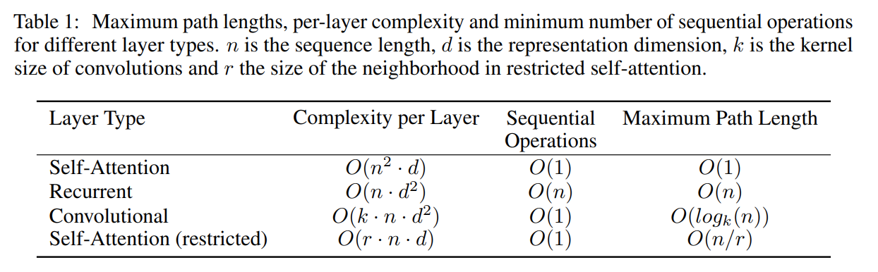
- Inspect Table 1 in Attention is all you Need with a focus on the “Complexity per Layer” column wherein n is the sequence length and d is the representation dimension, the same parameter as the self-attention projection size from Q1.
- Consider the complexity bounds and your own knowledge of how NLP tasks are constructed – describe when a self-attention network has a lower complexity than other networks.
- As a case study, we can set
d=1024and compare between these models. For most NLP tasks here we can approximate thatn << dand therefore the Transformer has lower complexity than the RNN. It might be helpful to name and discuss a few tasks where this is true. Conversely, there might be some cases where the inverse is true (document translation?). In terms of increasingn, the additional complexity in a Transformer makes sense as we need an additional self attention computation against all prior sequence elements. For the RNN, we only need to compute the RNN cell with the new state and cumulative history.
- As a case study, we can set
- Other than complexity – describe other constraining factors to be considered when planning experiments using neural networks for NLP. There is no right answer here.
- we now want to add in the practical other constraints that exist when running experiments. You could discuss that really this complexity is only a part of choosing models as well as performance and constraints such as GPU Memory, data availability, tunable hyperparameters etc. A typical Transformer is much larger than an RNN and space/speed constraints might arise before complexity can even be considered.
- Consider the complexity bounds and your own knowledge of how NLP tasks are constructed – describe when a self-attention network has a lower complexity than other networks.
- Consider an encoder-decoder RNN model, following up on the question before. Can the computation of the encoder be easily parallelised with respect to the number of tokens (meaning, can you break the input and the computation into chunks such that they run in parallel)? Explain why or why not.
- a
- Consider the Transformer encoder layer. Explain why its computation can be paralleised over tokens per layer. Can computation be easily parallelised across layers?
- a
- Considering Permutations
References
‘Transformers from scratch’ Available: https://peterbloem.nl/blog/transformers ↩︎
Tu, Zhaopeng, et al. “Neural machine translation with reconstruction.” Proceedings of the AAAI Conference on Artificial Intelligence. Vol. 31. No. 1. 2017. ↩︎
Koehn, Philipp, and Rebecca Knowles. “Six challenges for neural machine translation.” arXiv preprint arXiv:1706.03872 (2017). ↩︎
Holtzman, Ari, et al. “The curious case of neural text degeneration.” arXiv preprint arXiv:1904.09751 (2019). ↩︎
Vinyals, Oriol, et al. “Grammar as a foreign language.” Advances in neural information processing systems 28 (2015). ↩︎ ↩︎
Cao, Steven, Nikita Kitaev, and Dan Klein. “Unsupervised parsing via constituency tests.” arXiv preprint arXiv:2010.03146 (2020). ↩︎
Kaplan, Jared, et al. “Scaling laws for neural language models.” arXiv preprint arXiv:2001.08361 (2020). ↩︎
Hoffmann, Jordan, et al. “Training compute-optimal large language models.” arXiv preprint arXiv:2203.15556 (2022). ↩︎
Karpukhin, Vladimir, et al. “Dense Passage Retrieval for Open-Domain Question Answering.” EMNLP (1). 2020. ↩︎
Lewis, Patrick, et al. “Retrieval-augmented generation for knowledge-intensive nlp tasks.” Advances in neural information processing systems 33 (2020): 9459-9474. ↩︎