多臂老虎机问题(MAB)
符号&问题定义
- 大写斜体表示随机变量,例如$A, R, A_t, R_t$
- 小写字母表示这些随机变量的实现,例如$a, r, a_t, r_t, Pr${$A_t=a_t$}
- 花体,区间等表示集合,例如$\mathcal{A}, [0, 1], \mathbb{N}$
Given: a set of k actions, $\mathcal{A}$, number of rounds T. Repeat for t in T rounds:
- Algorithm selects arm $A_t \in \mathcal{A}$
- Algorithm observes reward $R_t \in [0, 1]$ Goal: maximise expected total reward.
预期的奖励被称为Value:$q_*(a) = \mathbb{E}[R_t \mid A_t = a]$
问题核心(Explore-exploit dilemma)
由于各个老虎机的奖励分布未知,我们需要在探索和利用之间做出权衡,来最大化长期奖励。
探索(Exploration) 和 利用(Exploitation) 之间的权衡是 MAB 问题的核心:
- Exploration: 选择当前信息不足的选项,以获得关于奖励分布的更多知识。例如,如果某个老虎机的奖励不确定,你可能会尝试拉取它,以收集更多数据。
- Exploitation: 选择当前估计奖励最高的选项,以最大化即时收益。例如,如果你已经知道某个老虎机的平均奖励最高,你会更倾向于持续拉取它。
这种权衡的核心难点在于:
- 过度探索(过多尝试未知选项)可能导致较低的短期收益。
- 过度利用(过早锁定某个选项)可能导致错失更优的长期收益。
问题算法
Action-Value Methods
我们可以估计某个动作$a$所获得奖励的样本均值。,具体函数表示为: $$ Q_t(a) = \frac{\text{Sum of rewards when taken a so far}}{\text{Number of times taken a so far}} $$ $$ Q_t(a) = \frac{1}{N_t(a)} \sum^{t-1}_{\tau=1}R _ {\tau=1} \cdot \mathbb{1} _ {A_t=a} $$ 其中
- $N_t(a)$ 是到当前时间 $t$ 为止,动作 $a$ 被选择的次数。
- $R_{\tau}$ 是第 $\tau$ 次执行动作的奖励。
- $\mathbb{1} _ {A_{\tau} = a}$ 是一个指示函数,当 $\tau$ 时刻选择了动作 $a$ 时,它的值为 1,否则为 0。
如果一个动作被选取无穷次,那么它的样本均值会收敛到真实的期望奖励,即: $$ \lim_{N_t(a) \to \infty} Q_t(a) = q_*(a) $$
$\epsilon$- Greedy Action Selection
根据上面的公式,我们可以把exploit表示为 $$ A_t = A_t^* = \mathop{\arg\max}\limits_{a} Q_t(a) $$ exploration(随机选择action)表示为 $$ A_t\sim\text{Unif}(\mathcal{A}) $$
def epsilon_greedy(Q, epsilon, actions):
    if np.random.rand() < epsilon:
        # 以概率 epsilon 进行探索
        return np.random.choice(actions)
    else:
        # 以概率 (1 - epsilon) 选择当前最优动作
        return np.argmax(Q)
    self.execute(A_t)
    self.observe(R_t)

    self.update(N_t_a, Q_t_a)
如何在递增的同时避免重复计算? $$ Q_n = \frac{R_1 + … + R_{n-1}}{n-1} $$ $$ Q_{n+1} = Q_n + \frac{1}{n}[R_n - Q_n] $$ 这也是强化学习中update rules的标准形式 $$ \text{NewEstimate <— OldEstimate + StepSize[Target - OldEstimate]} $$
Non-Stationary Problem
假设true action value会随时间而变化,这是强化学习中经常遇到的non-stationary problem,这个时候再用sample average就不合适了,我们引入一个step-size parameter $\alpha\in[0, 1]$来跟踪action value,那么更新函数变为 $$ Q_{n+1} = Q_n + \alpha[R_n - Q_n] $$
Stochastic Approximation Convergence Conditions
随机逼近(Stochastic Approximation, SA) 是一种用于在噪声环境中迭代逼近最优解的方法。它适用于我们无法直接求解目标函数的期望,只能通过带噪声的样本进行估计的情形。
在强化学习中,值函数更新 采用随机逼近的方式,例如: $$ Q_{t+1}(s, a) = Q_t(s, a) + \alpha_t [R_t + \gamma \max_{a’} Q_t(s’, a’) - Q_t(s, a)] $$ 其中 $\alpha_t$ 是学习率,目标是让 $Q_t(s,a)$ 收敛到最优值 $Q^*(s,a)$。
为了保证 随机逼近算法 能够收敛,必须满足收敛条件(Convergence Conditions):
学习率满足 Robbins-Monro 条件 $$ \sum_{t=1}^{\infty} \alpha_t = \infty, \quad \sum_{t=1}^{\infty} \alpha_t^2 < \infty $$
- 第一项 $ \sum \alpha_t = \infty $ 确保算法在长期内继续学习,否则算法可能过早停止更新。
- 第二项 $ \sum \alpha_t^2 < \infty $ 确保学习率最终足够小,否则收敛会受噪声影响。
示例:
- 满足条件的学习率: $ \alpha_t = \frac{1}{t} $、$ \alpha_t = \frac{1}{\sqrt{t}} $
- 不满足条件的学习率: 固定的 $ \alpha_t = 0.1 $(因为求和不发散)
Upper Confidence Bound (UCB)
相比于 $\epsilon$-Greedy 算法的随机探索策略,UCB 通过构造一个上置信界(Upper Confidence Bound)来进行探索,从而更快地收敛到最优解。
UCB 采用 置信区间(confidence bound) 来决定是否探索某个动作:
- 利用(Exploitation): 选择历史上平均奖励最高的动作(即当前最优动作)。
- 探索(Exploration): 选择那些尝试次数较少、不确定性较大的动作。
公式: $$ A_t = \arg\max_{a} \left[ Q_t(a) + c \sqrt{\frac{\ln t}{N_t(a)}} \right] $$ 其中:
- $ Q_t(a) $ 是动作 $ a $ 在时间 $ t $ 时刻的平均奖励(历史经验)。
- $ N_t(a) $ 是动作 $ a $ 被选择的次数。
- $ t $ 是当前时间步(当前实验的总次数)。
- $ c $ 是探索参数,控制探索程度(通常 $ c $ 取 $\sqrt{2}$)。
- $ \ln t $ 是对数项,使得探索随时间减少。
解释:
- $ Q_t(a) $ 代表 利用(Exploitation):倾向于选择历史上表现最好的动作。
- $ \sqrt{\frac{\ln t}{N_t(a)}} $ 代表 探索(Exploration):当某个动作选择次数$N_t(a)$很小时,该项较大,鼓励探索。
import numpy as np

def UCB(Q, N, t, c=1.0):
    ucb_values = Q + c * np.sqrt(np.log(t) / (N + 1e-5))  # 避免除零错误
    return np.argmax(ucb_values)  # 选择 UCB 值最高的动作
其中:
Q:存储每个动作的平均奖励。N:存储每个动作的选择次数。t:当前时间步数(总实验次数)。c:探索参数,控制探索强度。
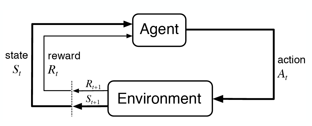
马尔可夫决策过程(MDPs)
理论框架
马尔可夫决策过程包括状态空间$\mathcal{S}$,动作空间$\mathcal{A}$,奖励空间$\mathcal{R}$。MDP是有限集,如果$\mathcal{S}$, $\mathcal{A}$, $\mathcal{R}$都是有限集
马尔可夫性质:简单说就是未来的状态只与当前一个状态有关,独立于过去的所有状态(Future state and reward are independent of past states and actions, given the current state and action)
$Pr${$S_{t+1},R_{t+1} | S_t,A_t,S_{t−1},A_{t−1},…,S_0,A_0$}$ = Pr${$S_{t+1},R_{t+1} | S_t,A_t$}
状态$S_t$是交互历史的充分总结。设计compact Markov states是RL中的一项工程工作。
以recycling robot为例。
- States
- high battery level
- low battery level
- Actions
- search for can
- wait for someone to bring can
- recharge battery at charging station
- Rewards: number of cans collected
| $s$ | $a$ | $s'$ | $p(s’\mid s, a)$ | $r(s, a, s’)$ |
|---|---|---|---|---|
| high | search | high | $\alpha$ | $r_{\text{research}}$ |
| high | search | low | $1 - \alpha$ | $r_{\text{research}}$ |
| low | search | high | $1 - \beta$ | -3 |
| low | search | low | $\beta$ | $r_{\text{research}}$ |
| high | wait | high | 1 | $r_{\text{wait}}$ |
| high | wait | low | 0 | - |
| low | wait | high | 0 | - |
| low | wait | low | 1 | $r_{\text{wait}}$ |
| high | recharge | high | 1 | 0 |
| high | recharge | low | 0 | - |
核心数学概念&函数
Policy
马尔可夫决策过程由policy控制。
$\pi(a\mid s) = $ 在状态$s$的情况下选择动作$a$的概率
| $\pi(a\mid s)$ | search | wait | recharge |
|---|---|---|---|
| high | 0.9 | 0.1 | 0 |
| low | 0.2 | 0.3 | 0.5 |
Agent的目标就是学一个能最大化累积奖励的策略
Returns(回报)
Total Return
策略应该最大化预期回报($G_t$) $$ G_t = R_{t+1} + R_{t+2} + … + R_{T} = R_{t+1} + G_{t+1} $$ where $T$ is final time step
Assumes terminating episodes: 适用于存在明确终止条件的任务。例如在象棋游戏中,一个玩家获胜就终止。通过设置允许的时间步数来强制终止
Discounted Return
对于不能终止的(无限的)场景,可以使用折扣率 $\gamma \in [0, 1)$ $$ G_t = R_{t+1} + \gamma R_{t+2} + \gamma^2 R_{t+3} + … = R_{t+1} + \gamma G_{t+1} $$ $\gamma$是折扣因子,用于降低远期奖励的价值。
这适用于无限回合任务,例如股票交易策略,智能体持续进行交易,没有固定结束时间。
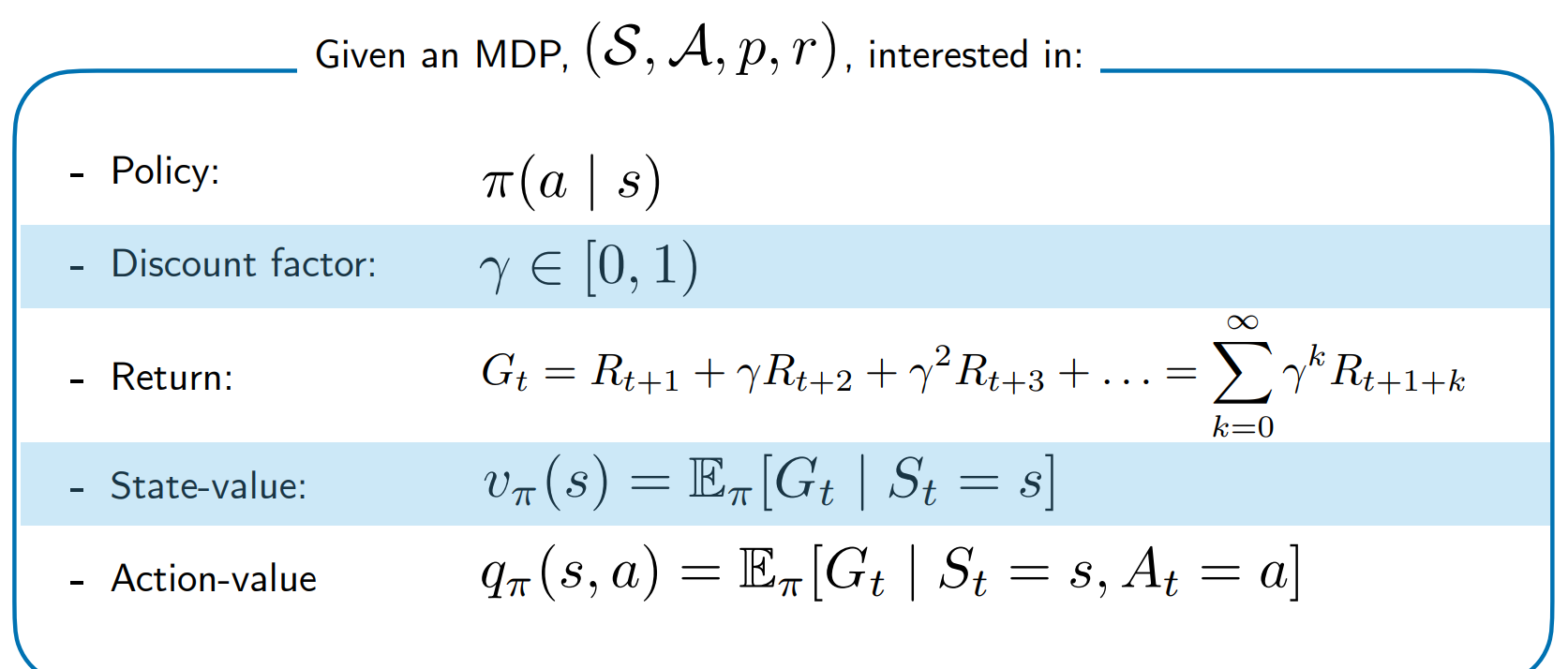
Value Functions
这张图给一个overview
 Bellman Equation
在强化学习和马尔可夫决策过程中,贝尔曼方程用于描述状态值函数和动作值函数的递归关系。这两是强化学习中求解最优策略的重要数学工具。
Bellman Equation
在强化学习和马尔可夫决策过程中,贝尔曼方程用于描述状态值函数和动作值函数的递归关系。这两是强化学习中求解最优策略的重要数学工具。
State Value Function and the Bellman Equation
根据Markov property,可以把状态价值函数写成Bellman Equation的递归形式。 $$ v_\pi(s) = \mathbb{E}_\pi[G_t \mid S_t = s] $$ 这个公式的意思就是给定当前状态的情况下,策略$\pi$可以获得的回报期望值
将公式展开,得到:
$$ v_\pi(s) = \sum_a \pi(a \mid s)r(s, a) + \gamma\sum_{s’ \in S} p(s’\mid s, a)\cdot v_\pi(s’) $$
其中$\sum_a \pi(a \mid s)r(s, a)$表示即时奖励(选择动作$a$的概率$\times$这样做带来的奖励值),$\gamma$是折扣因子,$\sum_{s’ \in S} p(s’\mid s, a)\cdot v_\pi(s’)$表示expected future value (当前状态$s$, 采取动作$a$之后,有多大概率转到每个可能的$s’$,每个$s’$会带来多大价值,全部加权求和后就是未来的预期价值)
直觉理解:眼前收益+未来收益(带有折扣率来降低影响)
Action Value Function的bellman形式 $$ q_\pi(s, a) = r(s, a) + \gamma \sum_{s’ \in S} p(s’ \mid s, a)\cdot v_\pi(s’) $$ 用期望简写 $$ q_\pi(s, a) = r(s, a) + \gamma \mathbb{E} _ {s’}[ v _ \pi(s’) ] $$
State value和action value有什么关系?
- state value是在某个状态下,按照策略$\pi$走下去,未来的期望总奖励
- action value是在某个状态下,执行动作$a$,再按照策略$\pi$走下去,未来的期望总奖励。
策略和动作的区别:策略不是动作的集合,而是一个“从状态到动作概率分布”的映射函数。
如果 $$ v _ \pi(s) = v_*(s) = \max_{\pi’}v_{\pi’}(s) $$
并且
$$ q_{\pi}(s, a) = q_*(s, a) = \max_{\pi’}q_{\pi’}(s, a) $$ 那么策略$\pi$就是最优的。
如何计算并找到这个最优策略?涉及到动态规划中的policy iteration和value iteration:
动态规划
动态规划核心思想:use Bellman Equations to organise search for good policies
DP Algo1: Policy Iteration
这个算法包含两个阶段:
- 策略评估:给定策略$\pi$, 计算对应的state value function $v_\pi(s)$; 解决Bellman方程,可迭代逼近
- 策略提升:用当前的$v_\pi(s)$来更新策略,如果新策略 = 旧策略,说明最优,停止。 $$ \pi_{\text{new}}(s) = \arg \max_a \sum_{s’}p(s’\mid s, a)[r(s, a) + \gamma v_\pi(s’)] $$
具体表示如下(这个过程会很快收敛到最优策略) $$ \pi_0 \xrightarrow{E} v_{\pi_0} \xrightarrow{I} \pi_1 \xrightarrow{E} v_{\pi_1} \xrightarrow{I} … \xrightarrow{I} \pi_* \xrightarrow{E} v_* $$
Iterative policy evaluation
伪代码如下
Input: pi, the policy to be evaluated
Initialize an array V(s) = 0, for all s
Repeat
    delta <- 0
    For each s in S:
        v <- V(s)
        V(s) <- State Value Function
        delta <- max(delta, |v - V(s)|)
until delta < theta (a small positive number)
Output V \approx= v_pi
Policy Improvement
计算在当前state value funtion $V(s)$下,每个状态$s$对不同动作$a$的action value。然后选择最优动作$\pi’(s)$,如果这与之前的$\pi(s)$不同,则策略发生了更新,并继续迭代,否则停止。
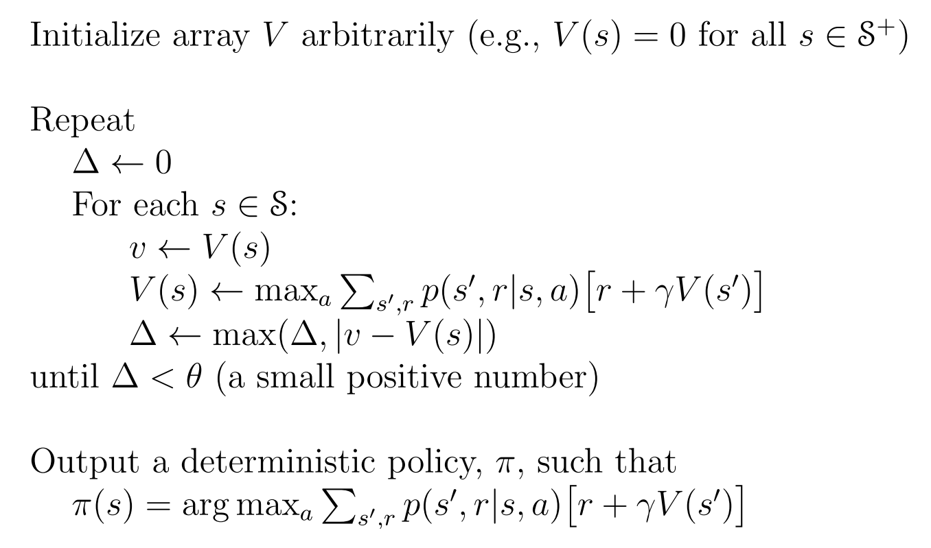
DP Algo2: Value Iteration
以租车问题为例。有两个车辆租赁点,根据分布随机请求和返回车辆。状态(States)表示为(n1, n2),其中ni是位置i的汽车数量(每个地方最多20辆)。动作(Actions)表示从一个位置移动到另一个位置的车子的数量。其中如果是从1移到2就是正数,从2移到1就是负数,最多5辆。奖励(Rewards)表示为每个时间步中,租出去一辆车+$10,移动一辆车-$2。最后$\gamma$ = 0.9。
Policy iteration使用Bellman equation作为operator: $$ v_{k+1}(s) = \sum_a \pi(a\mid s)\sum_{s’, r}p(s’, r\mid s, a) [r+\gamma v_k(s’)] $$ 其中$s\in S$
Value iteration使用Bellman optimality equation作为operator: $$ v_{k+1}(s) = \max_a \sum_{s’, r}p(s’, r\mid s, a) [r+\gamma v_k(s’)] $$ 其中$s\in S$
Value iteration的伪代码如下
Asynchronous and generalised DP
目前为止,动态规划方法执行的是穷举。如果状态空间很大,policy evaluation and improvement就不可计算了。
异步动态规划方法避免了标准动态规划中必须同时更新所有状态的限制,而是选择性地更新某些状态,以提高计算效率和收敛速度。
改进点:
- 状态异步更新:不要求所有状态在同一时间更新,而是按需更新一部分状态。
- 优先级更新:优先更新那些 价值变化较大或与最终策略最相关的状态,使有价值的信息更快传播。
- 加速收敛:减少不必要的计算,特别适用于大规模问题,如机器人控制、路径规划、强化学习等。
蒙特卡洛方法
Monte Carlo策略评估 - 在没有模型的情况下进行策略价值评估
MC不需要知道环境的模型$p(s’, r \mid s, a)$,只需要sampled episodes。你只需要能跟环境玩、玩完整场游戏,然后记录每个状态出现后最终赚了多少钱, 把这个“赚的钱”在所有访问过这个状态的 episode 里平均一下,这就是它的值$v_\pi(s)$。公式可以表示为 $$ v_\pi(s) = \mathbb{E} _ \pi[G_i \mid s_i = s] = \frac{1}{N(s)}\sum^{N(s)}_{i=1}G_i $$ 其中$N(s)$就是状态s被访问的次数,$G_i$是第i次访问s后的实际return。
s可能被多次访问,因此蒙特卡洛方法分为first-visit MC和every-visit MC。两者的区别在于更新时是否校验$S_t$已经在当前episode中出现过。First-visit只更新该状态第一次出现的位置,Every-visit则是该状态出现几次就更新几次。
如果无法得到环境的模型,那么计算动作的价值(“状态-动作”二元组的价值)比计算状态的价值更加有用。只需将对状态的访问改为对“状态-动作”二元组的访问,蒙特卡洛算法就可以几乎和之前完全相同的方式解决该问题,唯一复杂之处在于一些“状态-动作”二元组可能永远不会被访问到。为了实现基于动作价值函数的策略评估,我们必须保证持续的试探。一种方式是将指定的“状态-动作”二元组作为起点开始一幕采样,同时保证所有“状态-动作”二元组都有非零的概率可以被选为起点。这样就保证了在采样的幕个数趋于无穷时,每一个“状态-动作”二元组都会被访问到无数次。我们把这种假设称为MC control with exploring starts。
策略改进的方法是在当前价值函数上贪心地选择动作。由于我们有动作价值函数,所以在贪心的时候完全不需要使用任何的模型信息。对于任意的一个动作价值函数$q$, 对应的贪心策略为:对于任意一个状态$s\in S$, 必定选择对应动作价值函数最大的动作:$\pi(s) = \arg\max_a q(s, a)$
Exploring starts的一个重要假设是环境必须支持任意(s,a)起点,这在实际中几乎不成立。
但是现实中,我们很难满足试探性出发的假设,一般性的解法是智能体能够持续不断地选择所有可能的动作,有两种方法可以保证这一点,同轨策略(soft on-policy)和离轨策略(off-policy)。在同轨策略中,用于生成采样数据序列的策略和用于实际决策的待评估和改进的策略是相同的;而在离轨策略中,用于评估或改进的策略与生成采样数据的策略是不同的,即生成的数据“离开”了待优化的策略所决定的决策序列轨迹。
同轨策略
策略一般是软的,会逐渐逼近一个确定性的策略
离轨策略 所有的学习控制方法都面临一个困境:它们希望学到的动作可以使随后的智能体行为是最优的,但是为了搜索所有的动作(以保证找到最优动作),它们需要采取非最优的行动。离轨策略采用一种妥协的方法,它并不学习最优策略的动作值,而是学习一个接近最优而且仍能进行试探的策略的动作值。一个更加直接的方法是采用两个策略,一个用来学习并成为最优策略,另一个更加有试探性,用来产生智能体的行动样本。用来学习的策略被称为目标策略,用于生成行动样本的策略被称为行动策略。在这种情况下,我们认为学习所用的数据“离开”了待学习的目标策略,因此整个过程称为离轨策略学习。
Temporal Difference Learning
TD policy evaluation
利用时序差分方法解决控制问题,我们依然采用广义Policy Iteration,只是在评估和预测部分采用时序差分方法。同蒙特卡洛方法一样,我们需要在试探和开发之间做出权衡,因此方法又划分为同轨策略和离轨策略。
TD control
Sarsa
同轨策略下的TD。
On-policy中,我们需要对所有状态$s$以及动作$a$估计出在当前策略下所有对应的$q_\pi(s,a)$。确保state value在TD(0)下收敛的定理同样适用于在对应的action-value的算法上。 $$ Q(S_t, A_t) \leftarrow Q(S_t, A_t) + \alpha[R_{t+1} + \gamma Q(S_{t+1}, A_{t+1}) - Q(S_t, A_t)] $$ 每当从非终止状态的$S_t$出现一次转移之后,就进行上述的一次更新,如果$S_{t+1}$是终止状态,那么$Q(S_{t+1}, A_{t+1})$则定义为0。这个更新规则用到了$(S_t, A_t, R_{t+1}, S_{t+1}, A_{t+1})$,这也是为什么这个算法叫做Sarsa。
Q-learning
离轨策略下的TD
$$ Q(S_t, A_t) \leftarrow Q(S_t, A_t) + \alpha[R_{t+1} + \gamma \max_a Q(S_{t+1}, a) - Q(S_t, A_t)] $$ 在这里,待学习的action value函数$Q$采用了对最优动作价值函数$q_*$的直接近似作为学习目标,而与用于生成智能体决策序列轨迹的action policy是什么无关。
所以,Sarsa和Q-learning不仅在评估,而且还在改进策略。
Cliff Walking
用经典的悬崖行走问题来对比Sarsa和Q-Learning在策略学习上的差异。
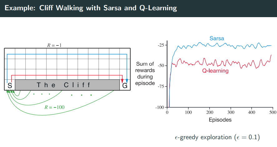 场景是这样,起点是S,终点是G,中间灰色是悬崖区域,一旦掉进去就-100然后重回起点,其他区域每一步奖励-1,每一步都用$\epsilon$-greedy来选择action。
在训练过程中,Sarsa更新的是自己实际经历的轨迹上的$Q(s, a)$, 因为它是On-policy,所以它避免靠近悬崖边,以防止$\epsilon$探索时不小心掉进去。结果是学到一个更保守但更稳定的路径(图中蓝色轨迹),牺牲了一点效率,但回报更高更稳定。
Q-learning更新的是理想中的最优策略(用最大的Q更新,哪怕当前没执行这个策略)。它学出来的策略更激进,会选择贴着悬崖走(图中红线),因为理论上这是最短路径、能最快到达终点、减少累计-1奖励。但现实中它使用$\epsilon$-greedy探索,一不小心探索出错就掉悬崖,得-100。所以虽然路径理论最优,但训练中平均回报更差、更不稳定。
n-steps TD methods
之前的TD(0)指的是只用一步未来信息(1 step return)的TD方法,问题是更新信息短浅,可能误差较大。但是如果考虑全部步数,就是一整个episode,就变成MC了。所以折中,这里介绍n-steps TD。
$$ V(S_t) \leftarrow V(S_t) + \alpha (G_{t:t+n} - V(S_t)) $$ 其中 $$ G_{t:t+n} = R_{t+1} + \gamma R_{t+2} + … + \gamma ^{n-1}R_{t+n} + \gamma^n V(S_{t+n}) $$
- 前n步使用的是真实奖励
- 第n+1步使用估计值
Planning and Learning
Dynamic Q-Learning
Value function approximation
Policy Gradient Methods
Reference
[1] https://leovan.me/cn/2020/07/model-free-policy-prediction-and-control-monte-carlo-learning/
[2] https://leovan.me/cn/2020/07/model-free-policy-prediction-and-control-temporal-difference-learning/